Inada conditions

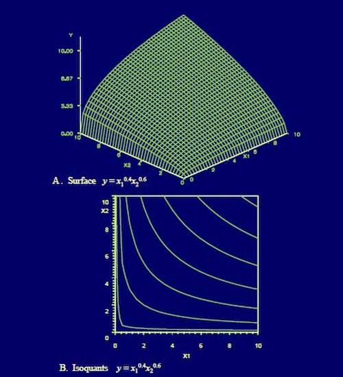
In macroeconomics, the Inada conditions are a set of mathematical assumptions about the shape and boundary behaviour of production or utility functions that ensure well-behaved properties in economic models, such as diminishing marginal returns and proper boundary behavior, which are essential for the stability and convergence of several macroeconomic models. The conditions are named after Ken-Ichi Inada, who introduced them in 1963.^[1][2] These conditions are typically imposed in neoclassical growth models — such as the Solow–Swan model, the Ramsey–Cass–Koopmans model, and overlapping generations models — to ensure that marginal returns are positive but diminishing, and that the marginal product of an input becomes infinite when its quantity approaches zero and vanishes when its quantity becomes infinitely large.

Economically, these properties guarantee well-behaved model dynamics: they rule out “corner solutions” such as zero capital accumulation or unbounded growth, ensure the existence of a unique and stable steady state, and promote smooth substitution between inputs. A Cobb–Douglas production function satisfies the Inada conditions, while some constant elasticity of substitution (CES) functions do not. Although stylized and not strictly realistic, the conditions are mathematically convenient and widely used in theoretical work because they simplify the analysis of long-run convergence and stability in dynamic macroeconomic models.

The Inada conditions are commonly associated with preventing pathological behaviors in production functions, such as infinite or zero capital accumulation.

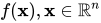
Given a continuously differentiable function ${\displaystyle f\colon X\to Y}$, where ${\displaystyle X=\left\{x\colon \,x\in \mathbb {R} _{+}^{n}\right\}}$ and ${\displaystyle Y=\left\{y\colon \,y\in \mathbb {R} _{+}\right\}}$, the conditions are:

1. the value of the function ${\displaystyle f(\mathbf {x} )}$ at ${\displaystyle \mathbf {x} =\mathbf {0} }$ is 0: ${\displaystyle f(\mathbf {0} )=0}$
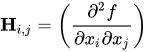
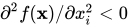
2. the function is concave on ${\displaystyle X}$, i.e. the Hessian matrix${\displaystyle \mathbf {H} _{i,j}=\left({\frac {\partial ^{2}f}{\partial x_{i}\partial x_{j}}}\right)}$ needs to be negative-semidefinite.^[3] Economically this implies that the marginal returns for input ${\displaystyle x_{i}}$ are positive, i.e. ${\displaystyle \partial f(\mathbf {x} )/\partial x_{i}>0}$, but decreasing, i.e. ${\displaystyle \partial ^{2}f(\mathbf {x} )/\partial x_{i}^{2}<0}$
3. the limit of the first derivative is positive infinity as ${\displaystyle x_{i}}$ approaches 0: ${\displaystyle \lim _{x_{i}\to 0}\partial f(\mathbf {x} )/\partial x_{i}=+\infty }$, meaning that the effect of the first unit of input ${\displaystyle x_{i}}$ has the largest effect
4. the limit of the first derivative is zero as ${\displaystyle x_{i}}$ approaches positive infinity: ${\displaystyle \lim _{x_{i}\to +\infty }\partial f(\mathbf {x} )/\partial x_{i}=0}$, meaning that the effect of one additional unit of input ${\displaystyle x_{i}}$ is 0 when approaching the use of infinite units of ${\displaystyle x_{i}}$

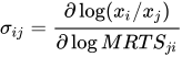
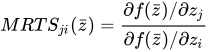
The elasticity of substitution between goods is defined for the production function ${\displaystyle f(\mathbf {x} ),\mathbf {x} \in \mathbb {R} ^{n}}$ as ${\displaystyle \sigma _{ij}={\frac {\partial \log(x_{i}/x_{j})}{\partial \log MRTS_{ji}}}}$, where ${\displaystyle MRTS_{ji}({\bar {z}})={\frac {\partial f({\bar {z}})/\partial z_{j}}{\partial f({\bar {z}})/\partial z_{i}}}}$ is the marginal rate of technical substitution. It can be shown that the Inada conditions imply that the elasticity of substitution between components is asymptotically equal to one (although the production function is not necessarily asymptotically Cobb–Douglas, a commonplace production function for which this condition holds).^[4][5]

In stochastic neoclassical growth model, if the production function does not satisfy the Inada condition at zero, any feasible path converges to zero with probability one, provided that the shocks are sufficiently volatile.^[6]

• Barro, Robert J.; Sala-I-Martin, Xavier I. (2004). Economic Growth (Second ed.). London: MIT Press. pp. 26–30. ISBN 0-262-02553-1.
• Gandolfo, Giancarlo (1996). Economic Dynamics (Third ed.). Berlin: Springer. pp. 176–178. ISBN 3-540-60988-1.
• Romer, David (2011). "The Solow Growth Model". Advanced Macroeconomics (Fourth ed.). New York: McGraw-Hill. pp. 6–48. ISBN 978-0-07-351137-5.

References

- ↑Inada, Ken-Ichi (1963). "On a Two-Sector Model of Economic Growth: Comments and a Generalization". The Review of Economic Studies. 30 (2): 119–127. doi:10.2307/2295809. JSTOR 2295809.
- ↑Uzawa, Hirofumi (1963). "On a Two-Sector Model of Economic Growth II". The Review of Economic Studies. 30 (2): 105–118. doi:10.2307/2295808. JSTOR 2295808.
- ↑Takayama, Akira (1985). Mathematical Economics (2nd ed.). New York: Cambridge University Press. pp. 125–126. ISBN 0-521-31498-4.
- ↑Barelli, Paulo; Pessoa, Samuel de Abreu (2003). "Inada Conditions Imply That Production Function Must Be Asymptotically Cobb–Douglas". Economics Letters. 81 (3): 361–363. doi:10.1016/S0165-1765(03)00218-0. hdl:10438/1012.
- ↑Litina, Anastasia; Palivos, Theodore (2008). "Do Inada conditions imply that production function must be asymptotically Cobb–Douglas? A comment". Economics Letters. 99 (3): 498–499. doi:10.1016/j.econlet.2007.09.035.
- ↑Kamihigashi, Takashi (2006). "Almost sure convergence to zero in stochastic growth models"(PDF). Economic Theory. 29 (1): 231–237. doi:10.1007/s00199-005-0006-1. S2CID 30466341.
Further reading