
Closed-loop transfer function
In control theory, a closed-loop transfer function is a mathematical function describing the net result of the effects of a feedback control loop on the input signal to the plant under control.
Overview
The closed-loop transfer function is measured at the output. The output signal can be calculated from the closed-loop transfer function and the input signal. Signals may be waveforms, images, or other types of data streams.
An example of a closed-loop block diagram, from which a transfer function may be computed, is shown below:
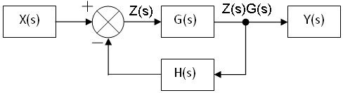
The summing node and the G(s) and H(s) blocks can all be combined into one block, which would have the following transfer function:
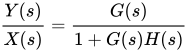
is called the feed forward transfer function, is called the feedback transfer function, and their product is called the open-loop transfer function.


Derivation
We define an intermediate signal Z (also known as error signal) shown as follows:
Using this figure we write:


Now, plug the second equation into the first to eliminate Z(s):
![{\displaystyle Y(s)=G(s)[X(s)-H(s)Y(s)]}](https://wikimedia.org/api/rest_v1/media/math/render/svg/28ca32117ca5a1061eb68777e15e264aae796d46)
Move all the terms with Y(s) to the left hand side, and keep the term with X(s) on the right hand side:

Therefore,

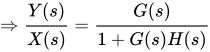
See also
References
 This article incorporates public domain material from Federal Standard 1037C. General Services Administration. Archived from the original on 2022-01-22.
- Classical control theory
- Cybernetics