
Explicit and implicit methods
Explicit and implicit methods are approaches used in numerical analysis for obtaining numerical approximations to the solutions of time-dependent ordinary and partial differential equations, as is required in computer simulations of physical processes. Explicit methods calculate the state of a system at a later time from the state of the system at the current time, while implicit methods find a solution by solving an equation involving both the current state of the system and the later one. Mathematically, if is the current system state and is the state at the later time ( is a small time step), then, for an explicit method



while for an implicit method one solves an equation

to find

Computation
Implicit methods require an extra computation (solving the above equation), and they can be much harder to implement. Implicit methods are used because many problems arising in practice are stiff, for which the use of an explicit method requires impractically small time steps to keep the error in the result bounded (see numerical stability). For such problems, to achieve given accuracy, it takes much less computational time to use an implicit method with larger time steps, even taking into account that one needs to solve an equation of the form (1) at each time step. That said, whether one should use an explicit or implicit method depends upon the problem to be solved.
Since the implicit method cannot be carried out for each kind of differential operator, it is sometimes advisable to make use of the so called operator splitting method, which means that the differential operator is rewritten as the sum of two complementary operators

while one is treated explicitly and the other implicitly. For usual applications the implicit term is chosen to be linear while the explicit term can be nonlinear. This combination of the former method is called Implicit-Explicit Method (short IMEX,[1][2][3]).
Illustration using the forward and backward Euler methods
Consider the ordinary differential equation
![{\displaystyle {\frac {dy}{dt}}=-y^{2},\ t\in [0,a]\quad \quad (2)}](https://wikimedia.org/api/rest_v1/media/math/render/svg/2da9a469600ad22b47c72ac29e5705592594d712)
with the initial condition This problem has the exact solution , which usually cannot be written down for problems encountered in practice, but in this case allows a comparison with the numerical solutions. Consider a grid for 0 ≤ k ≤ n, that is, the time step is and denote for each . قم بتقسيم هذه المعادلة باستخدام أبسط الطرق الصريحة والضمنية، وهي طرق أويلر الأمامية والخلفية (انظر المعادلات التفاضلية العادية العددية ) وقارن المخططات التي تم الحصول عليها.


- طريقة أويلر الأمامية

![{\displaystyle y'=-y^{2},\;t\in [0,5],\;y_{0}=1}](https://wikimedia.org/api/rest_v1/media/math/render/svg/3417b09298cdd5cb37559b2b094310257a20d2bf)

طريقة أويلر الأمامية
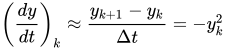
العائد

لكلهذه صيغة صريحة لـ.


- طريقة أويلر العكسية
باستخدام طريقة أويلر العكسية
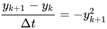
يجد المرء المعادلة الضمنية

ل(قارن هذا بالصيغة (3) حيث(تم إعطاؤها بشكل صريح بدلاً من كونها مجهولة في معادلة).
هذه معادلة تربيعية ، لها جذر سالب وجذر موجب . تم اختيار الجذر الموجب لأن الشرط الابتدائي في المعادلة الأصلية موجب، وبالتاليفي الخطوة الزمنية التالية يتم تحديدها بواسطة


في أغلب الحالات، تكون المعادلة المراد حلها باستخدام طريقة ضمنية أكثر تعقيدًا بكثير من المعادلة التربيعية، ولا يوجد لها حل تحليلي. عندئذٍ، تُستخدم خوارزميات إيجاد الجذور ، مثل طريقة نيوتن ، لإيجاد الحل العددي.
- طريقة كرانك-نيكلسون
باستخدام طريقة كرانك-نيكلسون

يجد المرء المعادلة الضمنية

ل(قارن هذا بالصيغة (3) حيث(تم إعطاؤها بشكل صريح بدلاً من كونها مجهولة في معادلة). يمكن حل ذلك عدديًا باستخدام خوارزميات إيجاد الجذور ، مثل طريقة نيوتن ، للحصول على.
يمكن اعتبار Crank-Nicolson شكلاً من أشكال مخططات IMEX ( الضمنية - الصريحة ) الأكثر عمومية.
- طريقة أويلر الأمامية والخلفية


لتطبيق مخطط IMEX، ضع في اعتبارك معادلة تفاضلية مختلفة قليلاً:
![{\displaystyle {\frac {dy}{dt}}=yy^{2},\ t\in [0,a]\quad \quad (5)}](https://wikimedia.org/api/rest_v1/media/math/render/svg/f18ea769b80c985190a3cdd00aab67ab5e172ee8)
ويترتب على ذلك أن
![{\displaystyle \left({\frac {dy}{dt}}\right)_{k}\approx y_{k+1}-y_{k}^{2},\ t\in [0,a]}](https://wikimedia.org/api/rest_v1/media/math/render/svg/7b04b3efd989e303c961793557c8ace14d9ab2d5)
وبالتالي

لكل
انظر أيضاً
- حالة كورانت-فريدريكس-ليوي
- خوارزمية SIMPLE ، وهي طريقة شبه ضمنية للمعادلات المرتبطة بالضغط
مصادر
- ↑ يو إم آشر، إس جيه روث، آر جيه سبيتيري: طرق رونج-كوتا الضمنية والصريحة للمعادلات التفاضلية الجزئية المعتمدة على الزمن ، الرياضيات العددية التطبيقية، المجلد 25 (2-3)، 1997
- ↑ L.Pareschi, G.Russo: Implicit-Explicit Runge-Kutta schemes for hard systems of differential equations , Recent Trends in Numerical Analysis, Vol. 3, 269-289, 2000
- ↑ سيباستيانو بوسكارينو، لورينزو باريسكي ، وجيوفاني روسو: طرق ضمنية-صريحة للمعادلات التفاضلية الجزئية التطورية ، SIAM، ISBN 978-1-61197-819-3 (2024).
- المعادلات التفاضلية العددية