حل منفرد

الحل الشاذ y ( _x ) لمعادلة تفاضلية عادية هو حل شاذ، أي حل لا يمتلك حلاً وحيداً لمسألة القيمة الابتدائية (والتي يسميها بعض الباحثين مسألة كوشي). قد تكون مجموعة الحلول الشاذة صغيرة كنقطة واحدة أو كبيرة كخط الأعداد الحقيقية بأكمله. ولا يشترط أن تكون الحلول الشاذة، بمعنى عدم امتلاك حل وحيد لمسألة القيمة الابتدائية، دوالاً شاذة .

في بعض الحالات، يُستخدم مصطلح "الحل الشاذ" للدلالة على حلٍّ لا يتحقق فيه التفرد لمسألة القيمة الابتدائية عند كل نقطة على المنحنى. يُعرَّف الحل الشاذ، بهذا المعنى الأعمق، بأنه مماس لكل حل من عائلة حلول. ونعني بالمماس وجود نقطة x حيث y _{_s} ( x ) = y _{_c} ( x ) و y' _{_s} ( x ) = y' _{_c} ( x )، حيث y _{_c} حلٌّ ضمن عائلة حلول مُعَلمة بالمعامل c . وهذا يعني أن الحل الشاذ هو غلاف عائلة الحلول.

عادةً ما تظهر الحلول الشاذة في المعادلات التفاضلية عند الحاجة إلى القسمة على حدٍّ قد يساوي صفرًا . لذا، عند حل معادلة تفاضلية باستخدام القسمة، يجب التحقق مما يحدث إذا كان الحدّ يساوي صفرًا، وما إذا كان يؤدي إلى حلٍّ شاذ. يمكن استخدام نظرية بيكارد-ليندلوف ، التي تُقدّم شروطًا كافية لوجود حلول فريدة، لاستبعاد وجود حلول شاذة. بينما تُقدّم نظريات أخرى، مثل نظرية بيانو للوجود ، شروطًا كافية لوجود حلول دون اشتراط أن تكون فريدة، مما قد يسمح بوجود حلول شاذة.

لنفترض المعادلة التفاضلية الخطية العادية المتجانسة

${\displaystyle xy'(x)+2y(x)=0,\,\!}$

حيث تشير العلامات (') إلى المشتقات بالنسبة إلى x . الحل العام لهذه المعادلة هو

${\displaystyle y(x)=Cx^{-2}.\,\!}$

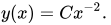
بالنسبة لـ${\displaystyle C}$هذا الحل سلس باستثناء عند${\displaystyle x=0}$حيث يكون الحل متباعداً. علاوة على ذلك، بالنسبة لقيمة معينة${\displaystyle x\not =0}$هذا هو الحل الفريد الذي يتم اتباعه${\displaystyle (x,y(x))}$.

لننظر في المعادلة التفاضلية

${\displaystyle y'(x)^{2}=4y(x).\,\!}$

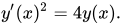
تُعطى عائلة من الحلول ذات المعامل الواحد لهذه المعادلة بواسطة

${\displaystyle y_{c}(x)=(xc)^{2}.\,\!}$

ويُقدّم حل آخر بواسطة

${\displaystyle y_{s}(x)=0.\,\!}$

Since the equation being studied is a first-order equation, the initial conditions are the initial x and y values. By considering the two sets of solutions above, one can see that the solution fails to be unique when ${\displaystyle y=0}$. (It can be shown that for ${\displaystyle y>0}$ if a single branch of the square root is chosen, then there is a local solution which is unique using the Picard–Lindelöf theorem.) Thus, the solutions above are all singular solutions, in the sense that solution fails to be unique in a neighbourhood of one or more points. (Commonly, we say "uniqueness fails" at these points.) For the first set of solutions, uniqueness fails at one point, ${\displaystyle x=c}$, and for the second solution, uniqueness fails at every value of ${\displaystyle x}$. Thus, the solution ${\displaystyle y_{s}}$ is a singular solution in the stronger sense that uniqueness fails at every value of x. However, it is not a singular function since it and all its derivatives are continuous.

In this example, the solution ${\displaystyle y_{s}(x)=0}$ is the envelope of the family of solutions ${\displaystyle y_{c}(x)=(xc)^{2}}$. The solution ${\displaystyle y_{s}}$ is tangent to every curve ${\displaystyle y_{c}(x)}$ at the point ${\displaystyle (c,0)}$.

The failure of uniqueness can be used to construct more solutions. These can be found by taking two constant ${\displaystyle c_{1}<c_{2}}$ and defining a solution ${\displaystyle y(x)}$ to be ${\displaystyle (x-c_{1})^{2}}$ when ${\displaystyle x<c_{1}}$, to be ${\displaystyle 0}$ when ${\displaystyle c_{1}\leq x\leq c_{2}}$, and to be ${\displaystyle (x-c_{2})^{2}}$ when ${\displaystyle x>c_{2}}$. Direct calculation shows that this is a solution of the differential equation at every point, including ${\displaystyle x=c_{1}}$ and ${\displaystyle x=c_{2}}$. Uniqueness fails for these solutions on the interval ${\displaystyle c_{1}\leq x\leq c_{2}}$, and the solutions are singular, in the sense that the second derivative fails to exist, at ${\displaystyle x=c_{1}}$ and ${\displaystyle x=c_{2}}$.

The previous example might give the erroneous impression that failure of uniqueness is directly related to ${\displaystyle y(x)=0}$. Failure of uniqueness can also be seen in the following example of a Clairaut's equation:

${\displaystyle y(x)=x\cdot y'+(y')^{2}\,\!}$

We write y' = p and then

${\displaystyle y(x)=x\cdot p+(p)^{2}.}$

Now, we shall take the differential according to x:

${\displaystyle p=y'=p+xp'+2pp'}$

which by simple algebra yields

${\displaystyle 0=(2p+x)p'.}$

This condition is solved if ${\displaystyle (2p+x)=0}$ or ${\displaystyle p'=0}$.

If p' = 0 it means that y' = p = c = constant, and the general solution of this new equation is:

${\displaystyle y_{c}(x)=c\cdot x+c^{2}}$

where c is determined by the initial value.

If x + 2p = 0 then we get that p = −½x and substituting in the ODE gives

${\displaystyle y_{s}(x)=(-{\tfrac {1}{2}}x)*x+(-{\tfrac {1}{2}}x)^{2}=-{\tfrac {1}{4}}x^{2}.}$

Now we shall check when these solutions are singular solutions. If two solutions intersect each other, that is, they both go through the same point (x,y), then there is a failure of uniqueness for a first-order ordinary differential equation. Thus, there will be a failure of uniqueness if a solution of the first form intersects the second solution.

شرط التقاطع هو  : y _s ( x ) = y _c ( x ). نحل

${\displaystyle c\cdot x+c^{2}=y_{c}(x)=y_{s}(x)=-{\tfrac {1}{4}}x^{2}}$

لإيجاد نقطة التقاطع، وهي${\displaystyle (-2c,-c^{2})}$.

يمكننا التحقق من أن المنحنيات متماسّة عند هذه النقطة _y 's ₍ x ) = y'c ( x ). نحسب المشتقات :

${\displaystyle y_{c}'(-2c)=c\,\!}$

${\displaystyle y_{s}'(-2c)=-{\tfrac {1}{2}}x|_{x=-2c}=c.\,\!}$

لذلك،

${\displaystyle y_{s}(x)=-{\tfrac {1}{4}}\cdot x^{2}\,\!}$

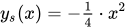
يكون مماساً لكل عضو من عائلة الحلول ذات المعامل الواحد

${\displaystyle y_{c}(x)=c\cdot x+c^{2}\,\!}$

من معادلة كليروت هذه:

${\displaystyle y(x)=x\cdot y'+(y')^{2}.\,\!}$

• معادلة تشاندراسيكار
• معادلة كريستال
• مادة كاوية (رياضيات)
• ظرف (رياضيات)
• مسألة القيمة الابتدائية
• نظرية بيكارد-ليندلوف

• روزوف، ن. خ. (2001) [1994]، "الحل الشاذ" ، موسوعة الرياضيات ، دار نشر EMS