Complex random vector 📅 آخر تحديث: ٣٠ يوليو ٢٠٢٦
✍️ نُشر في: ٣٠ يوليو ٢٠٢٦
📷 يحتوي على 69 صور
الموسوعة الحرة In probability theory and statistics , a complex random vector is typically a tuple of complex -valued random variables , and generally is a random variable taking values in a vector space over the field of complex numbers. If Z 1 , … , Z n {\displaystyle Z_{1},\ldots ,Z_{n}} n -tuple ( Z 1 , … , Z n ) {\displaystyle \left(Z_{1},\ldots ,Z_{n}\right)}
Some concepts of real random vectors have a straightforward generalization to complex random vectors. For example, the definition of the mean of a complex random vector. Other concepts are unique to complex random vectors.
Applications of complex random vectors are found in digital signal processing .
Definition A complex random vector Z = ( Z 1 , … , Z n ) T {\displaystyle \mathbf {Z} =(Z_{1},\ldots ,Z_{n})^{T}} probability space ( Ω , F , P ) {\displaystyle (\Omega ,{\mathcal {F}},P)} function Z : Ω → C n {\displaystyle \mathbf {Z} \colon \Omega \rightarrow \mathbb {C} ^{n}} ( ℜ ( Z 1 ) , ℑ ( Z 1 ) , … , ℜ ( Z n ) , ℑ ( Z n ) ) T {\displaystyle (\Re {(Z_{1})},\Im {(Z_{1})},\ldots ,\Re {(Z_{n})},\Im {(Z_{n})})^{T}} real random vector on ( Ω , F , P ) {\displaystyle (\Omega ,{\mathcal {F}},P)} ℜ ( z ) {\displaystyle \Re {(z)}} z {\displaystyle z} ℑ ( z ) {\displaystyle \Im {(z)}} z {\displaystyle z} [ 1] :
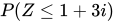
Cumulative distribution function The generalization of the cumulative distribution function from real to complex random variables is not obvious because expressions of the form P ( Z ≤ 1 + 3 i ) {\displaystyle P(Z\leq 1+3i)} P ( ℜ ( Z ) ≤ 1 , ℑ ( Z ) ≤ 3 ) {\displaystyle P(\Re {(Z)}\leq 1,\Im {(Z)}\leq 3)} F Z : C n ↦ [ 0 , 1 ] {\displaystyle F_{\mathbf {Z} }:\mathbb {C} ^{n}\mapsto [0,1]} Z = ( Z 1 , . . . , Z n ) T {\displaystyle \mathbf {Z} =(Z_{1},...,Z_{n})^{T}}
F Z ( z ) = P ( ℜ ( Z 1 ) ≤ ℜ ( z 1 ) , ℑ ( Z 1 ) ≤ ℑ ( z 1 ) , … , ℜ ( Z n ) ≤ ℜ ( z n ) , ℑ ( Z n ) ≤ ℑ ( z n ) ) {\displaystyle F_{\mathbf {Z} }(\mathbf {z} )=\operatorname {P} (\Re {(Z_{1})}\leq \Re {(z_{1})},\Im {(Z_{1})}\leq \Im {(z_{1})},\ldots ,\Re {(Z_{n})}\leq \Re {(z_{n})},\Im {(Z_{n})}\leq \Im {(z_{n})})} Eq.1
where z = ( z 1 , . . . , z n ) T {\displaystyle \mathbf {z} =(z_{1},...,z_{n})^{T}}
Expectation As in the real case the expectation (also called expected value ) of a complex random vector is taken component-wise.[ 1] :
E [ Z ] = ( E [ Z 1 ] , … , E [ Z n ] ) T {\displaystyle \operatorname {E} [\mathbf {Z} ]=(\operatorname {E} [Z_{1}],\ldots ,\operatorname {E} [Z_{n}])^{T}} Eq.2
Covariance matrix and pseudo-covariance matrix The covariance matrix second central moment ) K Z Z {\displaystyle \operatorname {K} _{\mathbf {Z} \mathbf {Z} }} n × 1 {\displaystyle n\times 1} n × n {\displaystyle n\times n} matrix whose ( i , j ) {\displaystyle (i,j)} th element is the covariance between the i th and the j th random variables.[ 2] : complex conjugate of one of the two. Thus the covariance matrix is a Hermitian matrix .[ 1] :
K Z Z = cov [ Z , Z ] = E [ ( Z − E [ Z ] ) ( Z − E [ Z ] ) H ] = E [ Z Z H ] − E [ Z ] E [ Z H ] {\displaystyle {\begin{aligned}&\operatorname {K} _{\mathbf {Z} \mathbf {Z} }=\operatorname {cov} [\mathbf {Z} ,\mathbf {Z} ]=\operatorname {E} [(\mathbf {Z} -\operatorname {E} [\mathbf {Z} ]){(\mathbf {Z} -\operatorname {E} [\mathbf {Z} ])}^{H}]=\operatorname {E} [\mathbf {Z} \mathbf {Z} ^{H}]-\operatorname {E} [\mathbf {Z} ]\operatorname {E} [\mathbf {Z} ^{H}]\\[12pt]\end{aligned}}}
Eq.3
K Z Z = [ E [ ( Z 1 − E [ Z 1 ] ) ( Z 1 − E [ Z 1 ] ) ¯ ] E [ ( Z 1 − E [ Z 1 ] ) ( Z 2 − E [ Z 2 ] ) ¯ ] ⋯ E [ ( Z 1 − E [ Z 1 ] ) ( Z n − E [ Z n ] ) ¯ ] E [ ( Z 2 − E [ Z 2 ] ) ( Z 1 − E [ Z 1 ] ) ¯ ] E [ ( Z 2 − E [ Z 2 ] ) ( Z 2 − E [ Z 2 ] ) ¯ ] ⋯ E [ ( Z 2 − E [ Z 2 ] ) ( Z n − E [ Z n ] ) ¯ ] ⋮ ⋮ ⋱ ⋮ E [ ( Z n − E [ Z n ] ) ( Z 1 − E [ Z 1 ] ) ¯ ] E [ ( Z n − E [ Z n ] ) ( Z 2 − E [ Z 2 ] ) ¯ ] ⋯ E [ ( Z n − E [ Z n ] ) ( Z n − E [ Z n ] ) ¯ ] ] {\displaystyle \operatorname {K} _{\mathbf {Z} \mathbf {Z} }={\begin{bmatrix}\mathrm {E} [(Z_{1}-\operatorname {E} [Z_{1}]){\overline {(Z_{1}-\operatorname {E} [Z_{1}])}}]&\mathrm {E} [(Z_{1}-\operatorname {E} [Z_{1}]){\overline {(Z_{2}-\operatorname {E} [Z_{2}])}}]&\cdots &\mathrm {E} [(Z_{1}-\operatorname {E} [Z_{1}]){\overline {(Z_{n}-\operatorname {E} [Z_{n}])}}]\\\\\mathrm {E} [(Z_{2}-\operatorname {E} [Z_{2}]){\overline {(Z_{1}-\operatorname {E} [Z_{1}])}}]&\mathrm {E} [(Z_{2}-\operatorname {E} [Z_{2}]){\overline {(Z_{2}-\operatorname {E} [Z_{2}])}}]&\cdots &\mathrm {E} [(Z_{2}-\operatorname {E} [Z_{2}]){\overline {(Z_{n}-\operatorname {E} [Z_{n}])}}]\\\\\vdots &\vdots &\ddots &\vdots \\\\\mathrm {E} [(Z_{n}-\operatorname {E} [Z_{n}]){\overline {(Z_{1}-\operatorname {E} [Z_{1}])}}]&\mathrm {E} [(Z_{n}-\operatorname {E} [Z_{n}]){\overline {(Z_{2}-\operatorname {E} [Z_{2}])}}]&\cdots &\mathrm {E} [(Z_{n}-\operatorname {E} [Z_{n}]){\overline {(Z_{n}-\operatorname {E} [Z_{n}])}}]\end{bmatrix}}} يتم تعريف مصفوفة التغاير الزائف مصفوفة العلاقة ) عن طريق استبدال النقل الهيرميتي بالنقل في التعريف أعلاه.
ج Z Z = كوف [ Z ، Z ¯ ] = هـ [ ( Z - هـ [ Z ] ) ( Z - هـ [ Z ] ) تي ] = هـ [ Z Z تي ] - هـ [ Z ] هـ [ Z تي ] {\displaystyle \operatorname {J} _{\mathbf {Z} \mathbf {Z} }=\operatorname {cov} [\mathbf {Z} ,{\overline {\mathbf {Z} }}]=\operatorname {E} [(\mathbf {Z} -\operatorname {E} [\mathbf {Z} ]){(\mathbf {Z} -\operatorname {E} [\mathbf {Z} ])}^{T}]=\operatorname {E} [\mathbf {Z} \mathbf {Z} ^{T}]-\operatorname {E} [\mathbf {Z} ]\operatorname {E} [\mathbf {Z} ^{T}]}
المعادلة 4
ج Z Z = [ هـ [ ( Z 1 - هـ [ Z 1 ] ) ( Z 1 - هـ [ Z 1 ] ) ] هـ [ ( Z 1 - هـ [ Z 1 ] ) ( Z 2 - هـ [ Z 2 ] ) ] ⋯ هـ [ ( Z 1 - هـ [ Z 1 ] ) ( Z ن - هـ [ Z ن ] ) ] هـ [ ( Z 2 - هـ [ Z 2 ] ) ( Z 1 - هـ [ Z 1 ] ) ] هـ [ ( Z 2 - هـ [ Z 2 ] ) ( Z 2 - هـ [ Z 2 ] ) ] ⋯ هـ [ ( Z 2 - هـ [ Z 2 ] ) ( Z ن - هـ [ Z ن ] ) ] ⋮ ⋮ ⋱ ⋮ هـ [ ( Z ن - هـ [ Z ن ] ) ( Z 1 - هـ [ Z 1 ] ) ] هـ [ ( Z ن - هـ [ Z ن ] ) ( Z 2 - هـ [ Z 2 ] ) ] ⋯ هـ [ ( Z ن - هـ [ Z ن ] ) ( Z ن - هـ [ Z ن ] ) ] ] {\displaystyle \operatorname {J} _{\mathbf {Z} \mathbf {Z} }={\begin{bmatrix}\mathrm {E} [(Z_{1}-\operatorname {E} [Z_{1}])(Z_{1}-\operatorname {E} [Z_{1}])]&\mathrm {E} [(Z_{1}-\operatorname {E} [Z_{1}])(Z_{2}-\operatorname {E} [Z_{2}])]&\cdots &\mathrm {E} [(Z_{1}-\operatorname {E} [Z_{1}])(Z_{n}-\operatorname {E} [Z_{n}])]\\\\\mathrm {E} [(Z_{2}-\operatorname {E} [Z_{2}])(Z_{1}-\operatorname {E} [Z_{1}])]&\mathrm {E} [(Z_{2}-\operatorname {E} [Z_{2}])(Z_{2}-\operatorname {E} [Z_{2}])]&\cdots &\mathrm {E} [(Z_{2}-\operatorname {E} [Z_{2}])(Z_{n}-\operatorname {E} [Z_{n}])]\\\\\vdots &\vdots &\ddots &\vdots \\\\\mathrm {E} [(Z_{n}-\operatorname {E} [Z_{n}])(Z_{1}-\operatorname {E} [Z_{1}])]&\mathrm {E} [(Z_{n}-\operatorname {E} [Z_{n}])(Z_{2}-\operatorname {E} [Z_{2}])]&\cdots &\mathrm {E} [(Z_{n}-\operatorname {E} [Z_{n}])(Z_{n}-\operatorname {E} [Z_{n}])]\end{bmatrix}}} ملكيات مصفوفة التغاير هي مصفوفة هيرميتية ، أي [ 1 ] :
ك Z Z ح = ك Z Z {\displaystyle \operatorname {K} _{\mathbf {Z} \mathbf {Z} }^{H}=\operatorname {K} _{\mathbf {Z} \mathbf {Z} }} مصفوفة التغاير الزائف هي مصفوفة متناظرة ، أي
ج Z Z تي = ج Z Z {\displaystyle \operatorname {J} _{\mathbf {Z} \mathbf {Z} }^{T}=\operatorname {J} _{\mathbf {Z} \mathbf {Z} }} مصفوفة التغاير هي مصفوفة شبه موجبة ، أي
أ ح ك Z Z أ ≥ 0 للجميع أ ∈ ج ن {\displaystyle \mathbf {a} ^{H}\operatorname {K} _{\mathbf {Z} \mathbf {Z} }\mathbf {a} \geq 0\quad {\text{for all }}\mathbf {a} \in \mathbb {C} ^{n}}
استقلال متجهان عشوائيان معقدانZ = ( Z 1 ، . . . ، Z م ) تي {\displaystyle \mathbf {Z} =(Z_{1},...,Z_{m})^{T}} دبليو = ( دبليو 1 ، . . . ، دبليو ن ) تي {\displaystyle \mathbf {W} =(W_{1},...,W_{n})^{T}} مستقلة إذا
F Z ، دبليو ( z ، w ) = F Z ( z ) ⋅ F دبليو ( w ) للجميع z ، w {\displaystyle F_{\mathbf {Z,W} }(\mathbf {z,w} )=F_{\mathbf {Z} }(\mathbf {z} )\cdot F_{\mathbf {W} }(\mathbf {w} )\quad {\text{for all }}\mathbf {z} ,\mathbf {w} } المعادلة 7
أينF Z ( z ) {\displaystyle F_{\mathbf {Z} }(\mathbf {z} )} F دبليو ( w ) {\displaystyle F_{\mathbf {W} }(\mathbf {w} )} Z {\displaystyle \mathbf {Z} } دبليو {\displaystyle \mathbf {W} } المعادلة 1 F Z ، دبليو ( z ، w ) {\displaystyle F_{\mathbf {Z,W} }(\mathbf {z,w} )} Z {\displaystyle \mathbf {Z} } دبليو {\displaystyle \mathbf {W} } Z ⊥ ⊥ دبليو {\displaystyle \mathbf {Z} \perp \!\!\!\perp \mathbf {W} } Z {\displaystyle \mathbf {Z} } دبليو {\displaystyle \mathbf {W} }
F Z 1 ، ... ، Z م ، دبليو 1 ، ... ، دبليو ن ( z 1 ، ... ، z م ، w 1 ، ... ، w ن ) = F Z 1 ، ... ، Z م ( z 1 ، ... ، z م ) ⋅ F دبليو 1 ، ... ، دبليو ن ( w 1 ، ... ، w ن ) للجميع z 1 ، ... ، z م ، w 1 ، ... ، w ن {\displaystyle F_{Z_{1},\ldots ,Z_{m},W_{1},\ldots ,W_{n}}(z_{1},\ldots ,z_{m},w_{1},\ldots ,w_{n})=F_{Z_{1},\ldots ,Z_{m}}(z_{1},\ldots ,z_{m})\cdot F_{W_{1},\ldots ,W_{n}}(w_{1},\ldots ,w_{n})\quad {\text{for all }}z_{1},\ldots ,z_{m},w_{1},\ldots ,w_{n}}
المتجهات العشوائية المركبة الصحيحة متجه عشوائي معقدZ {\displaystyle \mathbf {Z} } "صحيح" إذا تحققت الشروط الثلاثة التالية جميعها: [ 1 ] :
هـ [ Z ] = 0 {\displaystyle \operatorname {E} [\mathbf {Z} ]=0} متغير [ Z 1 ] < ∞ ، ... ، متغير [ Z ن ] < ∞ {\displaystyle \operatorname {var} [Z_{1}]<\infty ,\ldots ,\operatorname {var} [Z_{n}]<\infty } هـ [ Z Z تي ] = 0 {\displaystyle \operatorname {E} [\mathbf {Z} \mathbf {Z} ^{T}]=0} متجهان عشوائيان معقدانZ ، دبليو {\displaystyle \mathbf {Z} ,\mathbf {W} } المركبة بمتجهات مشتركة مناسبة إذا كانت متجهات عشوائية مركبة( Z 1 ، Z 2 ، ... ، Z م ، دبليو 1 ، دبليو 2 ، ... ، دبليو ن ) تي {\displaystyle (Z_{1},Z_{2},\ldots ,Z_{m},W_{1},W_{2},\ldots ,W_{n})^{T}}
ملكيات متجه عشوائي معقدZ {\displaystyle \mathbf {Z} } ج ∈ ج ن {\displaystyle \mathbf {c} \in \mathbb {C} ^{n}} ج تي Z {\displaystyle \mathbf {c} ^{T}\mathbf {Z} } [ 1 ] : التحويلات الخطية للمتجهات العشوائية المركبة الصحيحة تكون صحيحة، أي إذاZ {\displaystyle \mathbf {Z} } ن {\displaystyle n} أ {\displaystyle A} م × ن {\displaystyle m\times n} أ Z {\displaystyle A\mathbf {Z} } [ 1 ] : كل متجه عشوائي مركب متناظر دائريًا ذو تباين محدود لجميع مكوناته هو متجه حقيقي. [ 1 ] : توجد متجهات عشوائية مركبة حقيقية غير متناظرة دائريًا. [ 1 ] : يكون المتجه العشوائي الحقيقي صحيحاً إذا وفقط إذا كان ثابتاً. يكون متجهان عشوائيان مركبان صحيحان مشتركان غير مرتبطين إذا وفقط إذا كانت مصفوفة التغاير الخاصة بهما تساوي صفرًا، أي إذاك Z دبليو = 0 {\displaystyle \operatorname {K} _{\mathbf {Z} \mathbf {W} }=0}
متباينة كوشي -شفارتز للمتجهات العشوائية المعقدة هي
| هـ [ Z ح دبليو ] | 2 ≤ هـ [ Z ح Z ] هـ [ | دبليو ح دبليو | ] {\displaystyle \left|\operatorname {E} [\mathbf {Z} ^{H}\mathbf {W} ]\right|^{2}\leq \operatorname {E} [\mathbf {Z} ^{H}\mathbf {Z} ]\operatorname {E} [|\mathbf {W} ^{H}\mathbf {W} |]}
مراجع 1 2 3 4 5 6 7 8 9 10 لابيدوث، عاموس (2009). أساسيات الاتصال الرقمي . مطبعة جامعة كامبريدج. ISBN 978-0-521-19395-5 . ↑ غوبنر، جون أ. (2006). الاحتمالات والعمليات العشوائية لمهندسي الكهرباء والحاسوب . مطبعة جامعة كامبريدج. ISBN 978-0-521-86470-1 .1 2 3 تسي، ديفيد (2005). أساسيات الاتصالات اللاسلكية . مطبعة جامعة كامبريدج. فئات :
نظرية الاحتمالات العشوائية جبر المتغيرات العشوائية 









![{\displaystyle F_{\mathbf {Z} }:\mathbb {C} ^{n}\mapsto [0,1]}](https://wikimedia.org/api/rest_v1/media/math/render/svg/8661e6d29a4d779324e5c3978506838f8c244b65)



![{\displaystyle \operatorname {E} [\mathbf {Z} ]=(\operatorname {E} [Z_{1}],\ldots ,\operatorname {E} [Z_{n}])^{T}}](https://wikimedia.org/api/rest_v1/media/math/render/svg/9bad8687a134b34189596765316018f79fdca495)


![{\displaystyle {\begin{aligned}&\operatorname {K} _{\mathbf {Z} \mathbf {Z} }=\operatorname {cov} [\mathbf {Z} ,\mathbf {Z} ]=\operatorname {E} [(\mathbf {Z} -\operatorname {E} [\mathbf {Z} ]){(\mathbf {Z} -\operatorname {E} [\mathbf {Z} ])}^{H}]=\operatorname {E} [\mathbf {Z} \mathbf {Z} ^{H}]-\operatorname {E} [\mathbf {Z} ]\operatorname {E} [\mathbf {Z} ^{H}]\\[12pt]\end{aligned}}}](https://wikimedia.org/api/rest_v1/media/math/render/svg/ebd5472da7a2129480754c26bf1527c36e0e1aef)
![{\displaystyle \operatorname {K} _{\mathbf {Z} \mathbf {Z} }={\begin{bmatrix}\mathrm {E} [(Z_{1}-\operatorname {E} [Z_{1}]){\overline {(Z_{1}-\operatorname {E} [Z_{1}])}}]&\mathrm {E} [(Z_ {1}-\operatorname {E} [Z_{1}]){\overline {(Z_ {2}-\operatorname {E} [Z_{2}])}}]&\cdots &\mathrm {E} [(Z_{1}-\operatorname {E} [Z_{1}]){\overline {(Z_ {n}-\operatorname {E}) [Z_{n}])}}]\\\\\mathrm {E} [(Z_{2}-\اسم المشغل {E} [Z_{2}]){\overline {(Z_{1}-\اسم المشغل {E} [Z_{1}])}}]&\mathrm {E} [(Z_{2}-\اسم المشغل {E} [Z_{2}]){\overline {(Z_{2}-\اسم المشغل {E} [Z_{2}])}}]&\cdots &\mathrm {E} [(Z_{2}-\operatorname {E} [Z_{2}]){\overline {(Z_{n}-\operatorname {E} [Z_{n}])}}]\\\\\vdots &\vdots &\ddots &\vdots \\\\\mathrm {E} [(Z_{n}-\operatorname {E} [Z_{n}]){\overline {(Z_{1}-\operatorname {E} [Z_{1}])}}]&\mathrm {E} [(Z_ {n}-\operatorname {E} [Z_ {n}]) {\overline {(Z_ {2}-\operatorname {E} [Z_ {2}])}}]&\cdots &\mathrm {E} [(Z_ {n}-\operatorname {E}) [Z_ {n}]) {\overline {(Z_ {n} - \ اسم المشغل {E} [Z_ {n}])}}] \ end {bmatrix}}}](https://wikimedia.org/api/rest_v1/media/math/render/svg/445eafa0ab8d1d761c1c34d3bb993b4598ec4b15)
![{\displaystyle \operatorname {J} _{\mathbf {Z} \mathbf {Z} }=\operatorname {cov} [\mathbf {Z} ,{\overline {\mathbf {Z} }}]=\operatorname {E} [(\mathbf {Z} -\operatorname {E} [\mathbf {Z} ]){(\mathbf {Z} -\اسم المشغل {E} [\mathbf {Z} ])}^{T}]=\اسم المشغل {E} [\mathbf {Z} \mathbf {Z} ^{T}]-\اسم المشغل {E} [\mathbf {Z} ]\اسم المشغل {E} [\mathbf {Z} ^{T}]}](https://wikimedia.org/api/rest_v1/media/math/render/svg/073e290548d019170600567c2a29b7feaaf98a51)
![{\displaystyle \operatorname {J} _{\mathbf {Z} \mathbf {Z} }={\begin{bmatrix}\mathrm {E} [(Z_{1}-\operatorname {E} [Z_{1}])(Z_{1}-\operatorname {E} [Z_{1}])]&\mathrm {E} [(Z_{1}-\operatorname) {E} [Z_{1}])(Z_{2}-\operatorname {E} [Z_{2}])]&\cdots &\mathrm {E} [(Z_{1}-\operatorname {E} [Z_{1}])(Z_{n}-\operatorname {E} [Z_{n}])]\\\\\mathrm {E} [(Z_ {2}-\operatorname {ه} [Z_ {2}])(Z_{1}-\operatorname {E} [Z_{1}])]&\mathrm {E} [(Z_{2}-\operatorname {E} [Z_{2}])(Z_{2}-\operatorname {E} [Z_{2}])]&\cdots &\mathrm {E} [(Z_{2}-\operatorname {E}) [Z_ {2}])(Z_{n}-\operatorname {E} [Z_{n}])]\\\\\vdots &\ddots &\vdots \\\\\mathrm {E} [(Z_{n}-\operatorname {E} [Z_{n}])(Z_{1}-\operatorname {E} [Z_{1}])]&\mathrm {E} [(Z_{n}-\اسم المشغل {E} [Z_ {n}])(Z_{2}-\operatorname {E} [Z_{2}])]&\cdots &\mathrm {E} [(Z_{n}-\operatorname {E} [Z_{n}])(Z_{n}-\operatorname {E} [Z_{n}])]\end{bmatrix}}}](https://wikimedia.org/api/rest_v1/media/math/render/svg/50248ec68758163e693b5fa474537f0d953110ee)





![{\displaystyle {\begin{align}&\operatorname {K} _{\mathbf {X} \mathbf {X} }=\operatorname {E} [(\mathbf {X} -\operatorname {E} [\mathbf {X} ])(\mathbf {X} -\operatorname {E} [\mathbf {X} ])^{\mathrm {T} }]={\tfrac {1}{2}}\operatorname {Re} (\operatorname {K} _{\mathbf {Z} \mathbf {Z} }+\operatorname {J} _{\mathbf {Z} \mathbf {Z} })\\&\operatorname {K} _ {\mathbf {Y} \mathbf {Y} }=\operatorname {E} [(\mathbf {Y} -\operatorname {E} [\mathbf {Y} ])(\mathbf {Y} -\operatorname {E} [\mathbf {Y} ])^{\mathrm {T} }]={\tfrac {1}{2}}\operatorname {Re} (\operatorname {K} _ {\mathbf {Z} \mathbf {Z} }-\operatorname {J} _ {\mathbf {Z} \mathbf {Z} })\\&\operatorname {K} _{\mathbf {Y} \mathbf {X} }=\operatorname {E} [(\mathbf {Y} -\operatorname {E} [\mathbf {Y} ])(\mathbf {X} -\operatorname {E} [\mathbf {X}) ])^{\mathrm {T} }]={\tfrac {1}{2}}\operatorname {Im} (\operatorname {J} _{\mathbf {Z} \mathbf {Z} }+\operatorname {K} _{\mathbf {Z} \mathbf {Z} })\\&\operatorname {K} _ {\mathbf {X} \mathbf {Y} }=\operatorname {E} [(\mathbf {X} -\operatorname {E} [\mathbf {X} ])(\mathbf {Y} -\operatorname {E} [\mathbf {Y} ])^{\mathrm {T} }]={\tfrac {1}{2}}\operatorname {Im} (\operatorname {J} _ {\mathbf {Z} \mathbf {Z} }-\اسم المشغل {K} _{\mathbf {Z} \mathbf {Z} })\\\end{aligned}}}](https://wikimedia.org/api/rest_v1/media/math/render/svg/02b2d81c9eb40be718176122b197e7384c6ca81c)


![{\displaystyle \operatorname {K} _{\mathbf {Z} \mathbf {W} }=\operatorname {cov} [\mathbf {Z} ,\mathbf {W} ]=\operatorname {E} [(\mathbf {Z} -\operatorname {E} [\mathbf {Z} ]){(\mathbf {W} -\operatorname {E} [\mathbf {W} ])}^{H}]=\operatorname {E} [\mathbf {Z} \mathbf {W} ^{H}]-\operatorname {E} [\mathbf {Z} ]\operatorname {E} [\mathbf {W} ^{H}]}](https://wikimedia.org/api/rest_v1/media/math/render/svg/9844313bcca0b6e7e67e2c61bae3559a8714b4e4)
![{\displaystyle \operatorname {K} _{\mathbf {Z} \mathbf {W} }={\begin{bmatrix}\mathrm {E} [(Z_{1}-\operatorname {E} [Z_{1}]){\overline {(W_{1}-\operatorname {E} [W_{1}])}}]&\mathrm {E} [(Z_{1}-\اسم المشغل {E} [Z_{1}]){\overline {(W_{2}-\اسم المشغل {E} [W_{2}])}}]&\cdots &\mathrm {E} [(Z_{1}-\اسم المشغل {E} [Z_{1}]){\overline {(W_{n}-\اسم المشغل {E}) [W_{n}])}}]\\\\\mathrm {E} [(Z_{2}-\اسم المشغل {E} [Z_{2}]){\overline {(W_{1}-\اسم المشغل {E} [W_{1}])}}]&\mathrm {E} [(Z_{2}-\اسم المشغل {E} [Z_{2}]){\overline {(W_{2}-\اسم المشغل {E} [W_ {2}])}}]&\cdots &\mathrm {E} [(Z_{2}-\operatorname {E} [Z_{2}]){\overline {(W_{n}-\operatorname {E} [W_{n}])}}]\\\\\vdots &\vdots &\ddots &\vdots \\\\\mathrm {E} [(Z_{n}-\operatorname {E} [Z_{n}]){\overline {(W_{1}-\اسم المشغل {E} [W_{1}])}}]&\mathrm {E} [(Z_ {n}-\اسم المشغل {E} [Z_{n}]){\overline {(W_{2}-\اسم المشغل {E} [W_{2}])}}]&\cdots &\mathrm {E} [(Z_{n}-\اسم المشغل {E}) [Z_ {n}]) {\ overline {(W_ {n} - \ اسم المشغل {E} [W_ {n}])}}] \ end {bmatrix}}}](https://wikimedia.org/api/rest_v1/media/math/render/svg/9941690a38b08ff9f3b9be4bd1de0bb2fb9a67b5)
![{\displaystyle \operatorname {J} _{\mathbf {Z} \mathbf {W} }=\operatorname {cov} [\mathbf {Z} ,{\overline {\mathbf {W} }}]=\operatorname {E} [(\mathbf {Z} -\operatorname {E} [\mathbf {Z} ]){(\mathbf {W} -\اسم المشغل {E} [\mathbf {W} ])}^{T}]=\اسم المشغل {E} [\mathbf {Z} \mathbf {W} ^{T}]-\اسم المشغل {E} [\mathbf {Z} ]\اسم المشغل {E} [\mathbf {W} ^{T}]}](https://wikimedia.org/api/rest_v1/media/math/render/svg/3e6a151a8db17da379cb32babce0e737bca9a8b9)
![{\displaystyle \operatorname {J} _{\mathbf {Z} \mathbf {W} }={\begin{bmatrix}\mathrm {E} [(Z_{1}-\operatorname {E} [Z_{1}])(W_{1}-\operatorname {E} [W_{1}])]&\mathrm {E} [(Z_{1}-\operatorname) {E} [Z_{1}])(W_{2}-\اسم المشغل {E} [W_{2}])]&\cdots &\mathrm {E} [(Z_{1}-\اسم المشغل {E} [Z_{1}])(W_{n}-\اسم المشغل {E} [W_{n}])]\\\\\mathrm {E} [(Z_{2}-\اسم المشغل {ه} [Z_ {2}])(W_{1}-\operatorname {E} [W_{1}])]&\mathrm {E} [(Z_{2}-\operatorname {E} [Z_{2}])(W_{2}-\operatorname {E} [W_{2}])]&\cdots &\mathrm {E} [(Z_{2}-\operatorname {E}) [Z_ {2}])(W_{n}-\operatorname {E} [W_{n}])]\\\\\vdots &\ddots &\vdots \\\\\mathrm {E} [(Z_{n}-\operatorname {E} [Z_{n}])(W_{1}-\operatorname {E} [W_{1}])]&\mathrm {E} [(Z_{n}-\اسم المشغل {E} [Z_ {n}])(W_{2}-\operatorname {E} [W_{2}])]&\cdots &\mathrm {E} [(Z_{n}-\operatorname {E} [Z_{n}])(W_{n}-\operatorname {E} [W_{n}])]\end{bmatrix}}}](https://wikimedia.org/api/rest_v1/media/math/render/svg/240fc2c9717f84911d95a271d7ca87595b185cc5)










![{\displaystyle \operatorname {E} [\mathbf {Z} ]=0}](https://wikimedia.org/api/rest_v1/media/math/render/svg/d136e6dc4d72ba213940846421b1f8c00160bc8d)
![{\displaystyle \operatorname {var} [Z_{1}]<\infty ,\ldots ,\operatorname {var} [Z_{n}]<\infty }](https://wikimedia.org/api/rest_v1/media/math/render/svg/ca262a1fa11c0e897e89da432119076df0575dc4)
![{\displaystyle \operatorname {E} [\mathbf {Z} \mathbf {Z} ^{T}]=0}](https://wikimedia.org/api/rest_v1/media/math/render/svg/e567ff4fa3785973cc8d53106ec6a0e075d969e9)



![{\displaystyle \left|\operatorname {E} [\mathbf {Z} ^{H}\mathbf {W} ]\right|^{2}\leq \operatorname {E} [\mathbf {Z} ^{H}\mathbf {Z} ]\operatorname {E} [|\mathbf {W} ^{H}\mathbf {W} |]}](https://wikimedia.org/api/rest_v1/media/math/render/svg/e6675b4efe08db65ef119042110564db71520472)

![{\displaystyle \varphi _{\mathbf {Z} }(\mathbf {\omega } )=\operatorname {E} \left[e^{i\Re {(\mathbf {\omega } ^{H}\mathbf {Z} )}}\right]=\operatorname {E} \left[e^{i(\Re {(\omega _{1})}\Re {(Z_{1})}+\Im {(\omega _{1})}\Im {(Z_{1})}+\cdots +\Re {(\omega _{n})}\Re {(Z_{n})}+\Im {(\omega _{n})}\Im {(Z_{n})})}\right]}](https://wikimedia.org/api/rest_v1/media/math/render/svg/55ef4b68890cb6b51eea0081d9a757a4c9f88849)