Hamiltonian vector field

In mathematics and physics, a Hamiltonian vector field on a symplectic manifold is a vector field defined for any energy function or Hamiltonian. Named after the physicist and mathematician Sir William Rowan Hamilton, a Hamiltonian vector field is a geometric manifestation of Hamilton's equations in classical mechanics. The integral curves of a Hamiltonian vector field represent solutions to the equations of motion in the Hamiltonian form. The diffeomorphisms of a symplectic manifold arising from the flow of a Hamiltonian vector field are known as canonical transformations in physics and (Hamiltonian) symplectomorphisms in mathematics.^[1]

Hamiltonian vector fields can be defined more generally on an arbitrary Poisson manifold. The Lie bracket of two Hamiltonian vector fields corresponding to functions ${\displaystyle f}$ and ${\displaystyle g}$ on the manifold is itself a Hamiltonian vector field, with the Hamiltonian given by the Poisson bracket of ${\displaystyle f}$ and ${\displaystyle g}$.

Suppose that ${\displaystyle (M,\omega )}$ is a symplectic manifold. Since the symplectic form${\displaystyle \omega }$ is nondegenerate, it sets up a fiberwise-linearisomorphism

$${\displaystyle \omega :TM\to T^{*}M,}$$

between the tangent bundle${\displaystyle TM}$ and the cotangent bundle${\displaystyle T^{*}M}$, with the inverse

$${\displaystyle \Omega :T^{*}M\to TM,\quad \Omega =\omega ^{-1}.}$$

Therefore, one-forms on a symplectic manifold ${\displaystyle M}$ may be identified with vector fields and every differentiable function${\displaystyle H:M\rightarrow \mathbb {R} }$ determines a unique vector field${\displaystyle X_{H}}$, called the Hamiltonian vector field with the Hamiltonian${\displaystyle H}$, by defining for every vector field ${\displaystyle Y}$ on ${\displaystyle M}$,

$${\displaystyle \mathrm {d} H(Y)=\omega (X_{H},Y).}$$Or more succinctly, ${\displaystyle \iota _{X_{H}}\omega =dH}$.

Note: Some authors define the Hamiltonian vector field with the opposite sign. One has to be mindful of varying conventions in physical and mathematical literature.

Suppose that ${\displaystyle M}$ is a ${\displaystyle 2n}$-dimensional symplectic manifold. Then locally, one may choose canonical coordinates${\displaystyle (q^{1},\cdots ,q^{n},p_{1},\cdots ,p_{n})}$ on ${\displaystyle M}$, in which the symplectic form is expressed as:^[2]${\displaystyle \omega =\sum _{i}\mathrm {d} q^{i}\wedge \mathrm {d} p_{i},}$

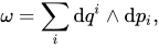
where ${\displaystyle \operatorname {d} }$ denotes the exterior derivative and ${\displaystyle \wedge }$ denotes the exterior product. Then the Hamiltonian vector field with Hamiltonian ${\displaystyle H}$ takes the form:^[1]${\displaystyle \mathrm {X} _{H}=\left({\frac {\partial H}{\partial p_{i}}},-{\frac {\partial H}{\partial q^{i}}}\right)=\Omega \,\mathrm {d} H,}$

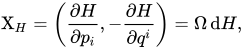
where ${\displaystyle \Omega }$ is a ${\displaystyle 2n\times 2n}$ square matrix

$${\displaystyle \Omega ={\begin{bmatrix}0&I_{n}\\-I_{n}&0\\\end{bmatrix}},}$$

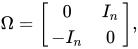
and

$${\displaystyle \mathrm {d} H={\begin{bmatrix}{\frac {\partial H}{\partial q^{i}}}\\{\frac {\partial H}{\partial p_{i}}}\end{bmatrix}}.}$$

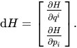
The matrix ${\displaystyle \Omega }$ is frequently denoted with ${\displaystyle \mathbf {J} }$.

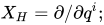
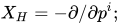
Suppose that ${\displaystyle M=\mathbb {R} ^{2n}}$ is the ${\displaystyle 2n}$-dimensional symplectic vector space with (global) canonical coordinates.

• If ${\displaystyle H=p_{i}}$ then ${\displaystyle X_{H}=\partial /\partial q^{i};}$
• if ${\displaystyle H=q_{i}}$ then ${\displaystyle X_{H}=-\partial /\partial p^{i};}$
• if ${\textstyle H={\frac {1}{2}}\sum (p_{i})^{2}}$ then ${\textstyle X_{H}=\sum p_{i}\partial /\partial q^{i};}$
• if ${\textstyle H={\frac {1}{2}}\sum a_{ij}q^{i}q^{j},a_{ij}=a_{ji}}$ then ${\textstyle X_{H}=-\sum a_{ij}q_{i}\partial /\partial p^{j}.}$

• The assignment ${\displaystyle f\mapsto X_{f}}$ is linear, so that the sum of two Hamiltonian functions transforms into the sum of the corresponding Hamiltonian vector fields.
• Suppose that ${\displaystyle (q^{1},\cdots ,q^{n},p_{1},\cdots ,p_{n})}$ are canonical coordinates on ${\displaystyle M}$ (see above). Then a curve ${\displaystyle \gamma (t)=(q(t),p(t))}$ is an integral curve of the Hamiltonian vector field ${\displaystyle X_{H}}$if and only if it is a solution of Hamilton's equations:^[1]$${\displaystyle {\begin{aligned}{\dot {q}}^{i}&={\frac {\partial H}{\partial p_{i}}}\\{\dot {p}}_{i}&=-{\frac {\partial H}{\partial q^{i}}}.\end{aligned}}}$$
• The Hamiltonian ${\displaystyle H}$ is constant along the integral curves, because ${\displaystyle \langle dH,{\dot {\gamma }}\rangle =\omega (X_{H}(\gamma ),X_{H}(\gamma ))=0}$. That is, ${\displaystyle H(\gamma (t))}$ is actually independent of ${\displaystyle t}$. This property corresponds to the conservation of energy in Hamiltonian mechanics.
• More generally, if two functions ${\displaystyle F}$ and ${\displaystyle H}$ have a zero Poisson bracket (cf. below), then ${\displaystyle F}$ is constant along the integral curves of ${\displaystyle H}$, and similarly, ${\displaystyle H}$ is constant along the integral curves of ${\displaystyle F}$. This fact is the abstract mathematical principle behind Noether's theorem.^{[nb 1]}
• The symplectic form${\displaystyle \omega }$ is preserved by the Hamiltonian flow. Equivalently, the Lie derivative${\displaystyle {\mathcal {L}}_{X_{H}}\omega =0}$.

The notion of a Hamiltonian vector field leads to a skew-symmetric bilinear operation on the differentiable functions on a symplectic manifold ${\displaystyle M}$, the Poisson bracket, defined by the formula

$${\displaystyle \{f,g\}=\omega (X_{g},X_{f})=dg(X_{f})={\mathcal {L}}_{X_{f}}g}$$

where ${\displaystyle {\mathcal {L}}_{X}}$ denotes the Lie derivative along a vector field ${\displaystyle X}$. Moreover, one can check that the following identity holds:^[1]${\displaystyle X_{\{f,g\}}=-[X_{f},X_{g}]}$,

where the right hand side represents the Lie bracket of the Hamiltonian vector fields with Hamiltonians ${\displaystyle f}$ and ${\displaystyle g}$. As a consequence (a proof at Poisson bracket), the Poisson bracket satisfies the Jacobi identity:^[1]${\displaystyle \{\{f,g\},h\}+\{\{g,h\},f\}+\{\{h,f\},g\}=0}$,

which means that the vector space of differentiable functions on ${\displaystyle M}$, endowed with the Poisson bracket, has the structure of a Lie algebra over ${\displaystyle \mathbb {R} }$, and the assignment ${\displaystyle f\mapsto X_{f}}$ is a Lie algebra homomorphism, whose kernel consists of the locally constant functions (constant functions if ${\displaystyle M}$ is connected).

• Hamiltonian vector field on nLab