Trochoidal wave

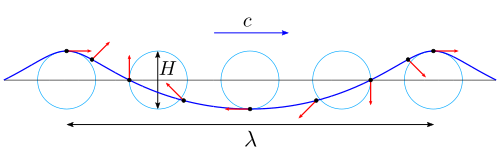
In fluid dynamics, a trochoidal wave or Gerstner wave is an exact solution of the Euler equations for periodicsurface gravity waves. It describes a progressive wave of permanent form on the surface of an incompressible fluid of infinite depth. The free surface of this wave solution is an inverted (upside-down) trochoid – with sharper crests and flat troughs. This wave solution was discovered by Gerstner in 1802, and rediscovered independently by Rankine in 1863.

The flow field associated with the trochoidal wave is not irrotational: it has vorticity. The vorticity is of such a specific strength and vertical distribution that the trajectories of the fluid parcels are closed circles. This is in contrast with the usual experimental observation of Stokes drift associated with the wave motion. Also the phase speed is independent of the trochoidal wave's amplitude, unlike other nonlinear wave-theories (like those of the Stokes wave and cnoidal wave) and observations. For these reasons – as well as for the fact that solutions for finite fluid depth are lacking – trochoidal waves are of limited use for engineering applications.

In computer graphics, the rendering of realistic-looking ocean waves can be done by use of so-called Gerstner waves. This is a multi-component and multi-directional extension of the traditional Gerstner wave, often using fast Fourier transforms to make (real-time) animation feasible.^[1]

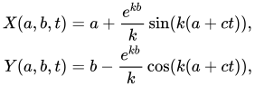
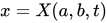
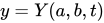
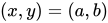
باستخدام مواصفات لاغرانجية لحقل التدفق ، تكون حركة جسيمات السائل – بالنسبة لموجة دورية على سطح طبقة سائلة ذات عمق لانهائي: ^{[ 2 ]}$${\displaystyle {\begin{aligned}X(a,b,t)&=a+{\frac {e^{kb}}{k}}\sin \left(k(a+ct)\right),\\Y(a,b,t)&=b-{\frac {e^{kb}}{k}}\cos \left(k(a+ct)\right),\end{aligned}}}$$ أين${\displaystyle x=X(a,b,t)}$و${\displaystyle y=Y(a,b,t)}$هي مواقع جزيئات السائل في${\displaystyle (x,y)}$الطائرة في ذلك الوقت${\displaystyle t}$، مع${\displaystyle x}$الإحداثي الأفقي و${\displaystyle y}$الإحداثي الرأسي (موجب لأعلى، في الاتجاه المعاكس للجاذبية). إحداثيات لاغرانج${\displaystyle (a,b)}$قم بتسمية أجزاء السائل، مع${\displaystyle (x,y)=(a,b)}$مراكز المدارات الدائرية - التي تتحرك حولها حزمة السائل المقابلة بسرعة ثابتة${\displaystyle c\,\exp(kb).}$إضافي${\textstyle k=2\pi /\lambda }$هو العدد الموجي (و${\displaystyle \lambda }$الطول الموجي )، بينما${\displaystyle c}$هي سرعة الطور التي تنتشر بها الموجة في${\displaystyle x}$في الاتجاه -. سرعة الطور تحقق علاقة التشتت : $${\displaystyle c^{2}={\frac {g}{k}},}$$ وهو مستقل عن اللاخطية الموجية (أي لا يعتمد على ارتفاع الموجة).${\displaystyle H}$) وسرعة هذه المرحلة${\displaystyle c}$وينطبق الأمر نفسه على الموجات الخطية التي شكلها آيري في المياه العميقة.

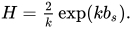
السطح الحر هو خط ضغط ثابت، وقد وُجد أنه يتوافق مع خط${\displaystyle b=b_{s}}$، أين${\displaystyle b_{s}}$هو ثابت (غير موجب). لـ${\displaystyle b_{s}=0}$تحدث أعلى الموجات، ذات قمة مدببة. لاحظ أن أعلى موجة ستوكس (غير الدورانية) لها زاوية قمة تبلغ 120 درجة، بدلاً من 0 درجة للموجة الدورانية الحلقية. ^{[ 3 ]}

ارتفاع موجة التروكويد هو${\textstyle H={\frac {2}{k}}\exp(kb_{s}).}$الموجة دورية في${\displaystyle x}$- في الاتجاه، بطول موجي${\displaystyle \lambda$ ;} وأيضًا دورية في الزمن بفترة زمنية${\textstyle T=\lambda /c={\sqrt {2\pi \lambda /g}}.}$

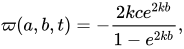
الدوامة​${\displaystyle \varpi }$تحت الموجة التروكويدية يوجد: ^{[ 2 ]}$${\displaystyle \varpi (a,b,t)=-{\frac {2kce^{2kb}}{1-e^{2kb}}},}$$ يختلف باختلاف الارتفاع اللاغرانجي${\displaystyle b}$ويتناقص بسرعة مع العمق تحت السطح الحر.

A multi-component and multi-directional extension of the Lagrangian description of the free-surface motion – as used in Gerstner's trochoidal wave – is used in computer graphics for the simulation of ocean waves.^[1] For the classical Gerstner wave the fluid motion exactly satisfies the nonlinear, incompressible and inviscid flow equations below the free surface. However, the extended Gerstner waves do in general not satisfy these flow equations exactly (although they satisfy them approximately, i.e. for the linearised Lagrangian description by potential flow). This description of the ocean can be programmed very efficiently by use of the fast Fourier transform (FFT). Moreover, the resulting ocean waves from this process look realistic, as a result of the nonlinear deformation of the free surface (due to the Lagrangian specification of the motion): sharper crests and flatter troughs.

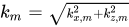
The mathematical description of the free-surface in these Gerstner waves can be as follows:^[1] the horizontal coordinates are denoted as ${\displaystyle x}$ and ${\displaystyle z}$, and the vertical coordinate is ${\displaystyle y}$. The mean level of the free surface is at ${\displaystyle y=0}$ and the positive ${\displaystyle y}$-direction is upward, opposing the Earth's gravity of strength ${\displaystyle g.}$ The free surface is described parametrically as a function of the parameters ${\displaystyle \alpha }$ and ${\displaystyle \beta ,}$ as well as of time ${\displaystyle t.}$ The parameters are connected to the mean-surface points ${\displaystyle (x,y,z)=(\alpha ,0,\beta )}$ around which the fluid parcels at the wavy surface orbit. The free surface is specified through ${\displaystyle x=\xi (\alpha ,\beta ,t),}$${\displaystyle y=\zeta (\alpha ,\beta ,t)}$ and ${\displaystyle z=\eta (\alpha ,\beta ,t)}$ with: $${\displaystyle {\begin{aligned}\xi &=\alpha -\sum _{m=1}^{M}{\frac {k_{x,m}}{k_{m}}}\,{\frac {a_{m}}{\tanh \left(k_{m}\,h\right)}}\,\sin \left(\theta _{m}\right),\\\eta &=\beta -\sum _{m=1}^{M}{\frac {k_{z,m}}{k_{m}}}\,{\frac {a_{m}}{\tanh \left(k_{m}\,h\right)}}\,\sin \left(\theta _{m}\right),\\\zeta &=\sum _{m=1}^{M}a_{m}\,\cos \left(\theta _{m}\right),\\\theta _{m}&=k_{x,m}\,\alpha +k_{z,m}\,\beta -\omega _{m}\,t-\phi _{m},\end{aligned}}}$$ where ${\displaystyle \tanh }$ is the hyperbolic tangent function, ${\displaystyle M}$ is the number of wave components considered, ${\displaystyle a_{m}}$ is the amplitude of component ${\displaystyle {m=1\dots M}}$ and ${\displaystyle \phi _{m}}$ its phase. Further ${\textstyle k_{m}={\sqrt {\scriptstyle k_{x,m}^{2}+k_{z,m}^{2}}}}$ is its wavenumber and ${\displaystyle \omega _{m}}$ its angular frequency. The latter two, ${\displaystyle k_{m}}$ and ${\displaystyle \omega _{m},}$ can not be chosen independently but are related through the dispersion relation: $${\displaystyle \omega _{m}^{2}=g\,k_{m}\tanh \left(k_{m}\,h\right),}$$ with ${\displaystyle h}$ the mean water depth. In deep water (${\displaystyle h\to \infty }$) the hyperbolic tangent goes to one: ${\displaystyle {\tanh(k_{m}\,h)\to 1.}}$ The components ${\displaystyle k_{x,m}}$ and ${\displaystyle k_{z,m}}$ of the horizontal wavenumber vector${\displaystyle {\boldsymbol {k}}_{m}}$ determine the wave propagation direction of component ${\displaystyle m.}$

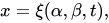
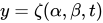
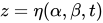
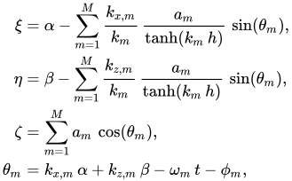
The choice of the various parameters ${\displaystyle a_{m},k_{x,m},k_{z,m}}$ and ${\displaystyle \phi _{m}}$ for ${\displaystyle m=1,\dots ,M,}$ and a certain mean depth ${\displaystyle h}$يُحدد شكل سطح المحيط. ويتطلب الأمر اختيارًا دقيقًا للاستفادة من إمكانية الحساب السريع باستخدام تحويل فورييه السريع (FFT). انظر على سبيل المثال Tessendorf (2001) للاطلاع على وصف لكيفية القيام بذلك. في أغلب الأحيان، يتم اختيار أرقام الموجات على شبكة منتظمة في${\displaystyle (k_{x},k_{z})}$-الفضاء. بعد ذلك، السعات${\displaystyle a_{m}}$والمراحل${\displaystyle \phi _{m}}$يتم اختيارها عشوائياً وفقاً لطيف كثافة التباين لحالة بحرية معينة مرغوبة . وأخيراً، باستخدام تحويل فورييه السريع (FFT)، يمكن بناء سطح المحيط بطريقة تجعله دورياً في المكان والزمان، مما يتيح التبليط - أي إنشاء دورية زمنية عن طريق إزاحة الترددات قليلاً.${\displaystyle \omega _{m}}$بحيث${\displaystyle \omega _{m}=m\,\Delta \omega }$ل${\displaystyle m=1,\dots ,M.}$

في عملية العرض، يتم أيضًا استخدام متجه العمودي${\displaystyle {\boldsymbol {n}}}$غالباً ما تكون هناك حاجة إلى الوصول إلى السطح. ويمكن حساب ذلك باستخدام الضرب الاتجاهي (${\displaystyle \times }$) مثل: $${\displaystyle {\boldsymbol {n}}={\frac {\partial {\boldsymbol {s}}}{\partial \alpha }}\times {\frac {\partial {\boldsymbol {s}}}{\partial \beta }}\quad {\text{with}}\quad {\boldsymbol {s}}(\alpha ,\beta ,t)={\begin{pmatrix}\xi (\alpha ,\beta ,t)\\\zeta (\alpha ,\beta ,t)\\\eta (\alpha ,\beta ,t)\end{pmatrix}}.}$$

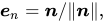
إذن ، يكون متجه الوحدة العمودي هو${\displaystyle {\boldsymbol {e}}_{n}={\boldsymbol {n}}/\|{\boldsymbol {n}}\|,}$مع${\displaystyle \|{\boldsymbol {n}}\|}$معيار​​${\displaystyle {\boldsymbol {n}}.}$