
المسار الجيوديسي

في الهندسة ، يُعرَّف الخط الجيوديسي ( يُلفظ /ˌdʒiː.əˈdɛsɪk , -oʊ- , -ˈdiːsɪk , -zɪk / ) [ 1 ] [ 2 ] بأنه منحنى يُمثل ، بمعنى ما ، أقصر مسار محليًا ( قوس ) بين نقطتين على سطح ، أو بشكل أعم، على مشعب ريماني . ويُستخدم المصطلح أيضًا في أي مشعب قابل للتفاضل مع اتصال . وهو تعميم لمفهوم " الخط المستقيم " .
يُشتق الاسم "جيوديسي" والصفة "جيوديسي" من علم الجيوديسيا ، وهو علم قياس حجم وشكل الأرض ، مع أن العديد من المبادئ الأساسية قابلة للتطبيق على أي شكل هندسي بيضاوي . في الأصل، كان الجيوديسي أقصر مسار بين نقطتين على سطح الأرض . بالنسبة للأرض الكروية ، فهو جزء من دائرة عظمى (انظر أيضًا مسافة الدائرة العظمى ). وقد عُمِّم المصطلح لاحقًا ليشمل فضاءات رياضية أكثر تجريدًا؛ على سبيل المثال، في نظرية المخططات ، يمكن اعتبار الجيوديسي بين رأسين /عقدتين في مخطط .
في فضاء ريماني أو فضاء فرعي ريماني، تتميز الخطوط الجيوديسية بخاصية انعدام انحنائها . وبشكل أعم، في وجود اتصال أفيني ، يُعرَّف الخط الجيوديسي بأنه منحنى تبقى متجهاته المماسية متوازية إذا نُقلت على طوله. بتطبيق هذا على اتصال ليفي-تشيفيتا لمقياس ريماني، يُستعاد المفهوم السابق.
تُعدّ الخطوط الجيوديسية ذات أهمية خاصة في النسبية العامة . وتصف الخطوط الجيوديسية الزمنية في النسبية العامة حركة جسيمات الاختبار الساقطة سقوطاً حراً .
مقدمة
يمكن تعريف أقصر مسار محلي بين نقطتين معطيتين في فضاء منحني، بافتراض أنه متعدد شعب ريماني، باستخدام معادلة طول المنحنى ( دالة f من فترة مفتوحة من R إلى الفضاء ) ، ثم تقليل هذا الطول بين النقطتين باستخدام حساب التفاضل والتكامل . يُعاني هذا من بعض المشاكل التقنية البسيطة نظرًا لوجود فضاء لانهائي الأبعاد من الطرق المختلفة لتمثيل أقصر مسار. من الأسهل حصر مجموعة المنحنيات بتلك التي تُمثل "بسرعة ثابتة" 1، أي أن المسافة من f ( s ) إلى f ( t ) على طول المنحنى تساوي | s - t |. وبالمثل، يمكن استخدام كمية مختلفة تُسمى طاقة المنحنى؛ يؤدي تقليل الطاقة إلى نفس المعادلات للمسار الجيوديسي (حيث "السرعة الثابتة" هي نتيجة للتقليل). يمكن فهم هذه الصيغة الثانية بشكل بديهي من خلال ملاحظة أن الشريط المطاطي المشدود بين نقطتين سيتقلص عرضه، وبالتالي سيقلل من طاقته. والشكل الناتج للشريط هو خط جيوديسي.
من الممكن أن تُقلل عدة منحنيات مختلفة المسافة بين نقطتين، كما هو الحال بالنسبة لنقطتين متقابلتين قطريًا على سطح الكرة. في هذه الحالة، يُعد أي من هذه المنحنيات خطًا جيوديسيًا.
الجزء المتصل من الخط الجيوديسي هو أيضاً خط جيوديسي.
بشكل عام، لا تُعدّ الخطوط الجيوديسية هي نفسها "أقصر المنحنيات" بين نقطتين، على الرغم من ترابط المفهومين. يكمن الفرق في أن الخطوط الجيوديسية تمثل أقصر مسافة بين النقاط محليًا فقط ، وتُحدد بمعامل "سرعة ثابتة". أما السير "في أطول مسار" على دائرة عظمى بين نقطتين على سطح الكرة فهو خط جيوديسي، ولكنه ليس أقصر مسار بين النقطتين. الخريطةإن الانتقال من الفترة 1 على خط الأعداد الحقيقية إلى نفسها يعطي أقصر مسار بين 0 و 1، ولكنه ليس مسارًا جيوديسيًا لأن سرعة الحركة المقابلة لنقطة ما ليست ثابتة.

تُستخدم الخطوط الجيوديسية بكثرة في دراسة الهندسة الريمانية ، وبشكل أعم في الهندسة المترية . في النسبية العامة ، تصف الخطوط الجيوديسية في الزمكان حركة الجسيمات النقطية تحت تأثير الجاذبية فقط. على وجه الخصوص، يُعد مسار صخرة ساقطة، أو قمر صناعي يدور في مدار ، أو شكل مدار كوكب ، جميعها خطوطًا جيوديسية في الزمكان المنحني. وبشكل أعم، يتناول موضوع الهندسة شبه الريمانية المسارات التي قد تسلكها الأجسام عندما لا تكون حرة الحركة، وتكون حركتها مقيدة بطرق مختلفة.
تُقدّم هذه المقالة الصياغة الرياضية المستخدمة في تعريف وإيجاد وإثبات وجود الخطوط الجيوديسية، في حالة المشعبات الريمانية. وتناقش مقالة " علاقة ليفي-تشيفيتا" الحالة الأكثر عمومية للمشعب الريماني الزائف والخط الجيوديسي (النسبية العامة) بتفصيل أكبر الحالة الخاصة للنسبية العامة.
أمثلة


من أكثر الأمثلة شيوعًا الخطوط المستقيمة في الهندسة الإقليدية . على سطح الكرة ، تُمثل الدوائر العظمى الخطوط الجيوديسية . أقصر مسار من النقطة أ إلى النقطة ب على سطح الكرة هو القوس الأقصر من الدائرة العظمى المار بالنقطتين أ و ب . إذا كانت أ و ب نقطتين متقابلتين ، فإنه يوجد عدد لا نهائي من أقصر المسارات بينهما. أما الخطوط الجيوديسية على سطح القطع الناقص فتتصرف بطريقة أكثر تعقيدًا من نظيرتها على سطح الكرة؛ فهي ليست مغلقة بشكل عام (انظر الشكل).
المثلثات
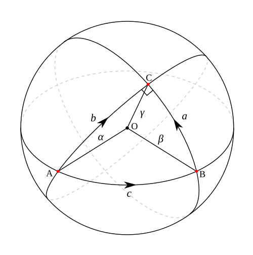
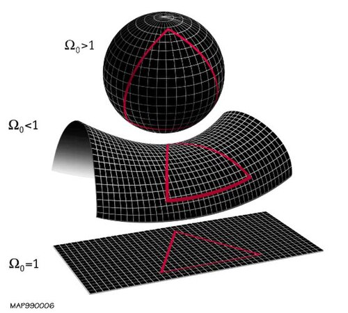
يتشكل المثلث الجيوديسي من خلال الخطوط الجيوديسية التي تربط كل زوج من النقاط الثلاث على سطح معين. أما على الكرة، فتكون الخطوط الجيوديسية عبارة عن أقواس دوائر عظمى ، لتشكل مثلثًا كرويًا .
الهندسة المترية
In metric geometry, a geodesic is a curve which is everywhere locally a distance minimizer. More precisely, a curveγ : I → M from an interval I of the reals to the metric spaceM is a geodesic if there is a constantv ≥ 0 such that for any t ∈ I there is a neighborhood J of t in I such that for any t1, t2 ∈ J we have

This generalizes the notion of geodesic for Riemannian manifolds. However, in metric geometry the geodesic considered is often equipped with natural parameterization, i.e. in the above identity v = 1 and

If the last equality is satisfied for all t1, t2 ∈ I, the geodesic is called a minimizing geodesic or shortest path.
In general, a metric space may have no geodesics, except constant curves. At the other extreme, any two points in a length metric space are joined by a minimizing sequence of rectifiable paths, although this minimizing sequence need not converge to a geodesic. The metric Hopf-Rinow theorem provides situations where a length space is automatically a geodesic space.
Common examples of geodesic metric spaces that are often not manifolds include metric graphs, (locally compact) metric polyhedral complexes, infinite-dimensional pre-Hilbert spaces, and real trees.
Riemannian geometry
In a Riemannian manifold with metric tensor, the length of a continuously differentiable curve :[a,b]\to M} is defined by


![{\displaystyle \gamma :[a,b]\to M}](https://wikimedia.org/api/rest_v1/media/math/render/svg/b5c2d8d0dd04be91ac24d40469cc8b8ad0c7057d)
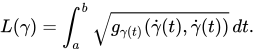
The distance between two points and of is defined as the infimum of the length taken over all continuous, piecewise continuously differentiable curves :[a,b]\to M} such that and . In Riemannian geometry, all geodesics are locally distance-minimizing paths, but the converse is not true. In fact, only paths that are both locally distance minimizing and parameterized proportionately to arc-length are geodesics.


Another equivalent way of defining geodesics on a Riemannian manifold, is to define them as the minima of the following action or energy functional

All minima of are also minima of , but is a bigger set since paths that are minima of can be arbitrarily re-parameterized (without changing their length), while minima of cannot. For a piecewise curve (more generally, a curve), the Cauchy–Schwarz inequality gives



with equality if and only if is equal to a constant a.e.; the path should be travelled at constant speed. It happens that minimizers of also minimize , because they turn out to be affinely parameterized, and the inequality is an equality. The usefulness of this approach is that the problem of seeking minimizers of is a more robust variational problem. Indeed, is a "convex function" of , so that within each isotopy class of "reasonable functions", one ought to expect existence, uniqueness, and regularity of minimizers. In contrast, "minimizers" of the functional are generally not very regular, because arbitrary reparameterizations are allowed.


The Euler–Lagrange equations of motion for the functional are then given in local coordinates by
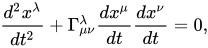
where are the Christoffel symbols of the metric. This is the geodesic equation, discussed below.

Calculus of variations
Techniques of the classical calculus of variations can be applied to examine the energy functional . The first variation of energy is defined in local coordinates by
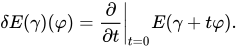
The critical points of the first variation are precisely the geodesics. The second variation is defined by

In an appropriate sense, zeros of the second variation along a geodesic arise along Jacobi fields. Jacobi fields are thus regarded as variations through geodesics.
By applying variational techniques from classical mechanics, one can also regard geodesics as Hamiltonian flows. They are solutions of the associated Hamilton equations, with (pseudo-)Riemannian metric taken as Hamiltonian.
Affine geodesics
A geodesic on a smooth manifold with an affine connection is defined as a curve such that parallel transport along the curve preserves the tangent vector to the curve, so


| 1 |

at each point along the curve, where is the derivative with respect to . More precisely, in order to define the covariant derivative of it is necessary first to extend to a continuously differentiable vector field in an open set. However, the resulting value of (1) is independent of the choice of extension.


استخدام الإحداثيات المحلية علىيمكننا كتابة معادلة الخط الجيوديسي (باستخدام اصطلاح الجمع ) على النحو التالي:
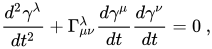
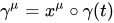
أينهي إحداثيات المنحنىوتُمثل رموز كريستوفيل الصلةهذه معادلة تفاضلية عادية للإحداثيات. ولها حل وحيد، بمعلومية الموضع الابتدائي والسرعة الابتدائية. لذلك، من وجهة نظر الميكانيكا الكلاسيكية ، يمكن اعتبار الخطوط الجيوديسية مسارات لجزيئات حرة في فضاء متعدد الأبعاد. في الواقع، المعادلةيعني هذا أن متجه تسارع المنحنى لا يحتوي على مركبات في اتجاه السطح (وبالتالي يكون عموديًا على المستوى المماس للسطح عند كل نقطة من المنحنى). لذا، فإن الحركة تتحدد كليًا بانحناء السطح. وهذه هي أيضًا فكرة النسبية العامة، حيث تتحرك الجسيمات على مسارات جيوديسية، ويكون الانحناء ناتجًا عن الجاذبية.
الوجود والتفرد
تنص نظرية الوجود المحلي والتفرد للخطوط الجيوديسية على أن الخطوط الجيوديسية على مشعب أملس ذي اتصال تآلفي موجودة، وهي فريدة. بتعبير أدق:
- لكل نقطة p في M ولكل متجه V في T p M ( الفضاء المماسي لـ M عند p ) يوجد خط جيوديسي وحيد : أنا → م بحيث
- و
- حيث I هي فترة مفتوحة قصوى في R تحتوي على 0.


يُستنتج برهان هذه النظرية من نظرية المعادلات التفاضلية العادية ، بملاحظة أن معادلة الجيوديسية هي معادلة تفاضلية عادية من الرتبة الثانية. ومن ثم، يُستنتج وجود الحل ووحدانيته من نظرية بيكارد-ليندلوف لحلول المعادلات التفاضلية العادية ذات الشروط الابتدائية المحددة. وتعتمد قيمة γ بسلاسة على كل من p و V.
بشكل عام، قد لا يكون I هو كل R كما هو الحال مثلاً بالنسبة لقرص مفتوح في R 2. أي γ يمتد إلى كل ℝ إذا وفقط إذا كانت M كاملة جيوديسياً .
التدفق الجيوديسي
التدفق الجيوديسي هو تأثير R محلي على الحزمة المماسية TM لمتشعب M مُعرَّف بالطريقة التالية
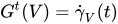
where t ∈ R, V ∈ TM and denotes the geodesic with initial data . Thus, is the exponential map of the vector tV. A closed orbit of the geodesic flow corresponds to a closed geodesic on M.



On a (pseudo-)Riemannian manifold, the geodesic flow is identified with a Hamiltonian flow on the cotangent bundle. The Hamiltonian is then given by the inverse of the (pseudo-)Riemannian metric, evaluated against the canonical one-form. In particular the flow preserves the (pseudo-)Riemannian metric , i.e.

In particular, when V is a unit vector, remains unit speed throughout, so the geodesic flow is tangent to the unit tangent bundle. Liouville's theorem implies invariance of a kinematic measure on the unit tangent bundle.
Geodesic spray
The geodesic flow defines a family of curves in the tangent bundle. The derivatives of these curves define a vector field on the total space of the tangent bundle, known as the geodesic spray.
More precisely, an affine connection gives rise to a splitting of the double tangent bundle TTM into horizontal and vertical bundles:

The double tangent bundle can be visualized as the space of simultaneous changes of both the base point and velocity, without committing to any method to transport velocity across base points.
For any , the vertical fiber is determined by the projection map . It consists of all ways to change the velocity while fixing the base point , and it is essentially a copy of translated from to . The affine connection then selects where would land under a change of base point while "fixing" velocity, which spans out the horizontal fiber . Conversely, given the split, transporting a vector along a trajectory simply means dragging the vector along the horizontal bundle, i.e. lifting the trajectory twice, from in to in to in , with the condition that .





The geodesic spray is the unique horizontal vector field W satisfying

at each point , here denotes the pushforward (differential) along the projection . Intuitively, discards the change to velocity and preserves change to base point.


بشكل أعم، يسمح نفس البناء بإنشاء حقل متجهي لأي اتصال إهرسمان على الحزمة المماسية. ولكي يكون الحقل المتجهي الناتج عبارة عن رذاذ (على الحزمة المماسية المحذوفة T M \ {0})، يكفي أن يكون الاتصال متغيرًا تحت عمليات إعادة التحجيم الموجبة، أي يكفي أن يكون، إذايتم نقلها بواسطةل، ثميجب نقلها إلىلأيليس بالضرورة أن يكون كذلك، إذاكما يتم نقلها إلى، ثميجب نقلها.


أي (انظر: اتصال إهرسمان# حزم المتجهات والمشتقات المتغيرة ) يكفي أن يحقق التوزيع الأفقي

لكل X ∈ T M \ {0} و λ > 0. هنا d ( S λ ) هو الدفع الأمامي على طول التماثل القياسي ومن الحالات الخاصة للاتصال غير الخطي الذي ينشأ بهذه الطريقة هو ذلك المرتبط بمتشعب فينسلر .

يُعدّ التباين في ظل عمليات إعادة التحجيم الموجبة ضروريًا لضمان أن يكون نقل المتجهات مُعرّفًا جيدًا على طول المسارات الموجهة، أي بالنظر إلى أي معلمات.من المنحنى، وأي "تغيير في التوقيت" متزايد بشكل رتيب تمامًا، المعايرة الجديدةلا يزال ينتج نفس نقل المتجهات. وبدون التكافؤ تحت عمليات إعادة التحجيم الموجبة، يعتمد نقل المتجهات على طول مسار موجه على المعلمات المحددة.


الخطوط الجيوديسية الأفينية والإسقاطية
المعادلة ( 1 ) ثابتة تحت إعادة التحديدات الخطية؛ أي، التحديدات من الشكل

حيث a و b عددان حقيقيان ثابتان. وبالتالي، فإنه بالإضافة إلى تحديد فئة معينة من المنحنيات المضمنة، تحدد معادلة الجيوديسية أيضًا فئة مفضلة من المعاملات على كل منحنى. وبناءً على ذلك، تُسمى حلول المعادلة ( 1 ) بالجيوديسيات ذات المعامل الأفيني .
يُحدد الاتصال الأفيني بمجموعة خطوطه الجيوديسية ذات المعاملات الأفينية، حتى الالتواء ( سبيفاك 1999 ، الفصل 6، الملحق الأول) . في الواقع، لا يؤثر الالتواء نفسه على مجموعة الخطوط الجيوديسية، لأن معادلة الخط الجيوديسي تعتمد فقط على الجزء المتناظر من الاتصال. بتعبير أدق، إذايوجد اتصالان بحيث يكون موتر الفرق


إذا كان متماثلًا معكوسًا ،ولها نفس المسارات الجيوديسية، بنفس المعاملات الأفينية. علاوة على ذلك، هناك اتصال فريد يجمعها بنفس المسارات الجيوديسية مثل ولكن مع التواء متلاشٍ.

يتم وصف المسارات الجيوديسية التي لا تخضع لمعاملات محددة بواسطة اتصال إسقاطي .
الأساليب الحسابية
Efficient solvers for the minimal geodesic problem on surfaces span several distinct approaches, including combinatorial wavefront propagation, direct numerical solution of the eikonal equation, and methods based on heat diffusion; the three methods below are representative rather than exhaustive.
Mitchell–Mount–Papadimitriou algorithm
Mitchell, Mount, and Papadimitriou addressed the discrete geodesic problem: finding the shortest path between two points on a triangulated polyhedral surface.[3] Their algorithm, often abbreviated MMP, uses a "continuous Dijkstra" approach, propagating a distance wavefront across the mesh in a manner analogous to Dijkstra's algorithm on a continuous domain; this wavefront's state on each edge is often described using the term "window."[4] MMP computes the exact geodesic distance and path in O(n2 log n) time and O(n2) space, where n is the number of edges of the surface.
Fast marching method
Kimmel and Sethian's fast marching method adapts to triangulated surfaces an eikonal-equation solver originally formulated on regular grids: a monotone upwind finite-difference scheme builds the distance function by sweeping outward from the source in order of increasing distance — a causality relationship analogous to Dijkstra's algorithm on a continuous domain.[5] It runs in O(n log n) time, where n is the number of mesh points, at the cost of only approximating the true geodesic distance. Later work further extended the fast-marching framework to implicit surfaces and point clouds.[6][7]
Heat method
Crane, Weischedel, and Wardetzky's heat method splits distance computation into two stages: first find the direction along which distance increases, then compute the distance itself.[8] The approach is motivated by Varadhan's formula, which relates the short-time behavior of the heat kernel to squared geodesic distance; applying that formula to a numerical approximation of the heat kernel, however, gives poor results, so the method instead uses only the direction of the diffused heat's gradient, normalizing it to obtain a unit vector field along geodesics. The distance function is then recovered by solving a Poisson equation against that field. Because both stages reduce to sparse linear systems that can be prefactored once, the method is well suited to repeated distance queries from different sources on a fixed mesh.
Ribbon test
A ribbon "test" is a way of finding a geodesic on a physical surface.[9] The idea is to fit a bit of paper around a straight line (a ribbon) onto a curved surface as closely as possible without stretching or squishing the ribbon (without changing its internal geometry).
For example, when a ribbon is wound as a ring around a cone, the ribbon would not lie on the cone's surface but stick out, so that circle is not a geodesic on the cone. If the ribbon is adjusted so that all its parts touch the cone's surface, it would give an approximation to a geodesic.
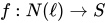
Mathematically the ribbon test can be formulated as finding a mapping of a neighborhood of a line in a plane into a surface so that the mapping "doesn't change the distances around by much"; that is, at the distance from we have where and are metrics on and .





Examples of applications
While geometric in nature, the idea of a shortest path is so general that it easily finds extensive use in nearly all sciences, and in some other disciplines as well.
Topology and geometric group theory
- In a surface with negative Euler characteristic, any (free) homotopy class determines a unique (closed) geodesic for a hyperbolic metric. These geodesics contribute significantly to the geometric understanding of the action of mapping classes.
- تتفاعل الفضاءات المترية الجيوديسية وفضاءات الطول بشكل ممتاز مع تأثيرات الزمر المتساوية القياس ( مثل مبرهنة شفارتس-ميلنور ، ومبرهنة هوبف-رينو ، ومبرهنة مورس، إلخ). وغالبًا ما تُشكّل هذه الفضاءات إطارًا مناسبًا لتعميم نتائج الهندسة الريمانية على الإنشاءات التي تعكس هندسة الزمرة. فعلى سبيل المثال، يمكن فهم خاصية غروموف-القطع الزائد من خلال رقة المثلثات الجيوديسية، ويمكن التعبير عن CAT(0) بدلالة الزوايا بين الجيوديسيات.
الاحتمالات والإحصاء والتعلم الآلي
- يمكن فهم النقل الأمثل على أنه مشكلة إيجاد المسارات الجيوديسية في فضاءات القياسات.
- في هندسة المعلومات ، تلعب التباعدات مثل تباعد كولباك-لايبير دورًا مشابهًا لدور المقياس الريماني، مما يسمح بإجراء مقارنات للاتصالات والجيوديسيات .
الفيزياء
- في الميكانيكا الكلاسيكية ، تُقلل المسارات الطاقة وفقًا لمعادلة هاميلتون-جاكوبي ، والتي يمكن اعتبارها فكرة مشابهة للجيوديسية. وفي بعض الحالات الخاصة، يتطابق المفهومان تمامًا .
- تُصوّر نظرية النسبية الزمكان على أنه متعدد الشعب اللورنتزي ، حيث يتبع الضوء الجيوديسيات اللورنتزي.
كيمياء
- في الكيمياء النظرية والحسابية ، يمكن حساب إحداثيات التفاعل الجوهرية لسطح طاقة الوضع (PES) كخط جيوديسي بين الحد الأدنى المحلي ( الحالات الوسيطة ) ونقاط السرج ( حالات الانتقال ). [ 10 ] [ 11 ]
- في الديناميكا الجزيئية ، يمكن التعامل مع تشكيلات البروتين كنقاط على سطح منحني، حيث تمثل الخطوط الجيوديسية أقصر المسارات وأقلها تشويهاً بين الهياكل، ويمكن أن تساعد في تقريب التحولات المرصودة والتفاعلات داخل الجزيئية. [ 12 ]
علم الأحياء
- يمكن تناول دراسة كيفية قيام الجهاز العصبي بتحسين الحركة العضلية من خلال تزويد فضاء تكوين الجسم بمقياس ريماني يقيس الجهد، بحيث يمكن صياغة المشكلة من حيث الجيوديسيا. [ 13 ]
- تُستخدم المسافة الجيوديسية غالبًا لقياس طول مسارات انتشار الإشارات في الخلايا العصبية. [ 14 ]
- تلعب هياكل الجيوديسية في الجزيئات الكبيرة دورًا في دراسة طيات البروتين . [ 15 ]
- [ 16 ] بنية العيون المركبة ، حيث يتم تثبيت ودعم أجزاء كثيرة منها بواسطة شبكة قبة جيوديسية على السطح الخارجي للعين.
هندسة
تُستخدم الخطوط الجيوديسية كأساس لحساب ما يلي:
- هياكل الطائرات الجيوديسية؛ انظر هيكل الطائرة الجيوديسي أو هيكل الطائرة الجيوديسي
- المسافات الأفقية على سطح الأرض أو بالقرب منها؛ انظر: الجيوديسيات الأرضية
- رسم الصور على الأسطح لأغراض العرض؛ انظر رسم الخرائط فوق البنفسجية
- تخطيط حركة الروبوت (على سبيل المثال، عند طلاء أجزاء السيارة)؛ انظر مشكلة أقصر مسار
- تصحيح أقصر مسار جيوديسي (GSP) على إعادة بناء سطح بواسون (مثلًا في طب الأسنان الرقمي )؛ بدون إعادة بناء GSP غالبًا ما ينتج عنه تقاطعات ذاتية داخل السطح
انظر أيضاً
- مقدمة في رياضيات النسبية العامة
- علاقة كليروت – صيغة في الهندسة التفاضلية الكلاسيكية. صفحات تعرض أوصافًا مختصرة للأهداف المعاد توجيهها.
- المنحنى القابل للتفاضل – دراسة المنحنيات من منظور تفاضلي
- الهندسة التفاضلية للأسطح
- الدائرة الجيوديسية
- نظرية هوبف – رينو – تعطي عبارات مكافئة حول اكتمال الخطوط الجيوديسية في مشعبات ريمان.
- المقياس الجوهري – مفهوم في الهندسة/الطوبولوجيا
- الخط المتساوي الخواص – الخط الذي تكون عنده قيمة الإزاحة التربيعية المطبقة على أي نقطتين تساوي صفرًا
- حقل جاكوبي – حقل متجه في الهندسة الريمانية
- نظرية مورس – تحلل طوبولوجيا متعدد الشعب من خلال دراسة الدوال القابلة للتفاضل على ذلك متعدد الشعب
- سطح زول – سطح متماثل الشكل مع الكرة
- مشكلة العنكبوت والذبابة – مشكلة الجيوديسيا الترفيهية
ملحوظات
- ↑ بالنسبة لنقطتين على الكرة ليستا متقابلتين، يوجد قوسان دائريان عظيمان بأطوال مختلفة يربطان بينهما، وكلاهما جيوديسي.
- 1 2 بالنسبة للمتشعب شبه الريماني ، على سبيل المثال، المتشعب اللورنتزي ، يكون التعريف أكثر تعقيدًا.
- ↑ المسار هو قيمة عظمى محلية للفترة k بدلاً من قيمة صغرى محلية.
مراجع
- ↑ "جيوديسي" . قاموس ليكسيكو الإنجليزي البريطاني . مطبعة جامعة أكسفورد . مؤرشف من الأصل بتاريخ 16-03-2020.
- ↑ "جيوديسي" . قاموس Merriam-Webster.com . Merriam-Webster. OCLC 1032680871 .
- ↑ ميتشل، ج.؛ ماونت، د.؛ باباديميتريو، س. (1987). "مسألة الجيوديسية المنفصلة" . مجلة SIAM للحوسبة . 16 (4): 647-668 . doi : 10.1137/0216045 .
- ↑ شين، س.-ك.؛ وانغ، ج.-ج. (2009). "تحسين خوارزمية تشين وهان في مسألة الجيوديسية المنفصلة". معاملات ACM في الرسومات . 28 (4): 104:1–104:8. doi : 10.1145/1559755.1559761 .
- ↑ كيميل، ر.؛ سيثيان، ج. أ. (1998). "حساب المسارات الجيوديسية على المشعبات" (ملف PDF) . وقائع الأكاديمية الوطنية للعلوم . 95 (15): 8431-8435 . رمز Bibcode : 1998PNAS...95.8431K . doi : 10.1073/pnas.95.15.8431 . PMC 21092. PMID 9671694. مؤرشف (ملف PDF) من الأصل بتاريخ 2022-10-09 .
- ↑ ميمولي، ف.؛ سابيرو، ج. (2001). "الحساب السريع لدوال المسافة الموزونة والجيوديسيات على الأسطح الفائقة الضمنية". مجلة الفيزياء الحاسوبية . 173 (2): 730-764 . doi : 10.1006/jcph.2001.6910 .
- ↑ ميمولي، ف.؛ سابيرو، ج. (2005). "دوال المسافة والجيوديسيات على الفضاءات الفرعية من R d والسحب النقطية". مجلة SIAM للرياضيات التطبيقية . 65 (4): 1227-1260 . doi : 10.1137/S003613990342877X .
- ↑ كرين، ك.؛ فايشيدل، س.؛ واردتزكي، م. (2017). "طريقة الحرارة لحساب المسافة" . اتصالات رابطة مكائن الحوسبة . 60 (11): 90-99 . doi : 10.1145/3131280 . S2CID 7078650 .
- ↑ Vsauce (2017-11-02). أي اتجاه هو الأسفل؟ . تم الاسترجاع في 2025-03-26 – عبر يوتيوب.
- ↑ أغيلار-موغاس، أنطوني؛ خيمينيز، خافيير؛ بوفيل، جوزيب ماريا (14 مارس 2008). "إيجاد مسارات التفاعل باستخدام طاقة الوضع كإحداثية للتفاعل". مجلة الفيزياء الكيميائية . 128 (10): 104102. doi : 10.1063/1.2834930 . ISSN 0021-9606 . PMID 18345872 .
- ↑ هايت، ديبتاركا؛ إسترادا بابون، جان د.؛ ستور، مارتن؛ مارتينيز، تود ج. (25-11-2025). "تحديد حالات الانتقال الأولية عبر بناء جيوديسي على أسطح طاقة كامنة مُتعلمة آليًا". مجلة نظرية الحساب الكيميائي . 21 (22): 11632-11644 . arXiv : 2507.17968 . doi : 10.1021/acs.jctc.5c01221 . ISSN 1549-9626 . PMID 41190940 .
- ↑ ديبيفين، ويليم؛ إستيف-ياغوي، كارلوس؛ ليلمان، يان؛ أوكتيم، أوزان؛ شونليب، كارولا-بيبيان (13 أغسطس 2024). " الهندسة الريمانية لتحليل بيانات ديناميكيات البروتين بكفاءة" . وقائع الأكاديمية الوطنية للعلوم في الولايات المتحدة الأمريكية . 121 (33) e2318951121. doi : 10.1073/pnas.2318951121 . ISSN 1091-6490 . PMC 11331106. PMID 39121160 .
- ↑ نيلسون، بيتر د.؛ نيلسون، ميغان د.؛ باي، روبن ت. (2015-12-01). "نظرية هندسية ريمانية لحركة الإنسان: فرضية التآزر الجيوديسي" . علم حركة الإنسان . 44 : 42-72 . doi : 10.1016/j.humov.2015.08.010 . ISSN 0167-9457 . PMID 26302481 .
- ↑ بيشكوف، كوسيو؛ تيسينغا، بول (2022-02-01). "المسافة القائمة على الجيوديسية تكشف عن خصائص طوبولوجية غير خطية في النشاط العصبي من القشرة البصرية للفأر" . علم التحكم الآلي البيولوجي . 116 (1): 53-68 . doi : 10.1007/s00422-021-00906-5 . ISSN 1432-0770 . PMID 34816322 .
- ↑ زانوتي، جوزيبي؛ غيرا، كونشيتينا (16 يناير 2003). "هل يُعدّ مفهوم التنسيغريتي مفهومًا موحدًا لطيات البروتين؟" . رسائل FEBS . 534 (1): 7-10 . Bibcode : 2003FEBSL.534....7Z . doi : 10.1016/S0014-5793(02)03853-X . ISSN 0014-5793 . PMID 12527354 .
- ^ كلاسين، فيليز؛ كروننبرج ، روبرت (10 مارس 2006). البيئات القابلة للنقل 3 . تايلور وفرانسيس. ص. 175. ردمك 978-1-134-28879-3.
- سبيفاك، مايكل (1999)، مقدمة شاملة في الهندسة التفاضلية (المجلد 2) ، هيوستن، تكساس: دار النشر Publish or Perish، رقم ISBN 978-0-914098-71-3
للمزيد من القراءة
- أدلر، رونالد؛ بازين، موريس؛ شيفر، مناحيم (1975)، مقدمة في النسبية العامة (الطبعة الثانية )، نيويورك: ماكجرو هيل ، ISBN 978-0-07-000423-8انظر الفصل الثاني .
- أبراهام، رالف هـ.؛ مارسدن ، جيرولد إي. (1978)، أسس الميكانيكا ، لندن: بنجامين-كامينغز، رمز Bibcode : 1978fome.book.....A ، ISBN 978-0-8053-0102-1انظر القسم 2.7 .
- جوست، يورغن (2002)، الهندسة الريمانية والتحليل الهندسي ، برلين، نيويورك: سبرينغر-فيرلاغ ، ISBN 978-3-540-42627-1انظر القسم 1.4 .
- كوباياشي، شوشيتشي ؛ نوميزو، كاتسومي (1996)، أسس الهندسة التفاضلية ، المجلد 1 ( طبعة جديدة)، وايلي-إنترساينس، ISBN 0-471-15733-3.
- لاندو، إل دي ؛ ليفشيتز، إي إم (1975)، النظرية الكلاسيكية للحقول ، أكسفورد: بيرغامون، رمز Bibcode : 1975ctf..book.....L ، ISBN 978-0-08-018176-9انظر القسم 87 .
- ميسنر، تشارلز دبليو ؛ ثورن، كيب ؛ ويلر، جون أرشيبالد (1973)، الجاذبية ، دبليو إتش فريمان، رقم ISBN 978-0-7167-0344-0
- أورتين ، توماس (2004)، الجاذبية والأوتار ، مطبعة جامعة كامبريدج ، ISBN 978-0-521-82475-0لاحظ بشكل خاص الصفحتين 7 و 10.
- فولكوف، يو. أ. (2001) [1994]، "الخط الجيوديسي" ، موسوعة الرياضيات ، دار نشر EMS.
- واينبرغ، ستيفن (1972)، الجاذبية وعلم الكونيات: مبادئ وتطبيقات النظرية النسبية العامة ، نيويورك: جون وايلي وأولاده ، رمز Bibcode : 1972gcpa.book.....W ، رقم ISBN 978-0-471-92567-5انظر الفصل 3 .
روابط خارجية
- إعادة النظر في الجيوديسيات - مقدمة عن الجيوديسيات بما في ذلك طريقتان لاشتقاق معادلة الجيوديسية مع تطبيقات في الهندسة (الجيوديسية على الكرة وعلى الطارة )، والميكانيكا ( البراكيستوكرون ) والبصريات (شعاع الضوء في وسط غير متجانس).
- مشعب فرعي جيوديسي بالكامل. مؤرشف بتاريخ 10 أغسطس 2015 في أرشيف الإنترنت (Wayback Machine) ضمن أطلس المشعبات.
- الهندسة التفاضلية
- الجيوديسية (الرياضيات)