
Norm (mathematics)
In mathematics, a norm is a function from a real or complex vector space to the non-negative real numbers that behaves in certain ways like the distance from the origin: it commutes with scaling, obeys a form of the triangle inequality, and is zero only at the origin. In particular, the Euclidean distance in a Euclidean space is defined by a norm on the associated Euclidean vector space, called the Euclidean norm, the 2-norm, or, sometimes, the magnitude or length of the vector. This norm can be defined as the square root of the inner product of a vector with itself.
A seminorm satisfies the first two properties of a norm but may be zero for vectors other than the origin.[1] A vector space with a specified norm is called a normed vector space. In a similar manner, a vector space with a seminorm is called a seminormed vector space.
The term pseudonorm has been used for several related meanings. It may be a synonym of "seminorm".[1] It can also refer to a norm that can take infinite values[2] or to certain functions parametrised by a directed set.[3]
Definition
Given a vector space over a subfield of the complex numbers a norm on is a real-valued function with the following properties, where denotes the usual absolute value of a scalar :[4]


- Subadditivity / Triangle inequality: for all
- Absolute homogeneity: for all and all scalars
- Positive definiteness / Positiveness[5] / Point-separating:for all if then
- Because property (2.) implies some authors replace property (3.) with the equivalent condition: for every if and only if





A seminorm on is a function that has properties (1.) and (2.)[6] so that in particular, every norm is also a seminorm (and thus also a sublinear functional). However, there exist seminorms that are not norms.
Properties (1.) and (2.) imply that if is a norm (or more generally, a seminorm), then and that also has the following property:[a]


- Non-negativity:[5] for all


Some authors include non-negativity as part of the definition of "norm", although this is not necessary. Although this article defined "positive" to be a synonym of "positive definite", some authors instead define "positive" to be a synonym of "non-negative";[7] these definitions are not equivalent.
Notation
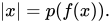
If a norm is given on a vector space then the norm of a vector is usually denoted by enclosing it within double vertical lines: , as proposed by Stefan Banach in his doctoral thesis from 1920. Such notation is also sometimes used if is only a seminorm. For the length of a vector in Euclidean space (which is an example of a norm, as explained below), the notation with single vertical lines is also widespread.


Examples
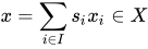
Every (real or complex) vector space admits a norm: If is a Hamel basis for a vector space then the real-valued map that sends (where all but finitely many of the scalars are ) to is a norm on [8] There are also a large number of norms that exhibit additional properties that make them useful for specific problems.



Absolute-value norm
The absolute value is a norm on the vector space formed by the real or complex numbers. The complex numbers form a one-dimensional vector space over themselves and a two-dimensional vector space over the reals, and the absolute value is a norm for these two structures. For example, 1 as the basis and the complex numbers as scalars form a 1-dimensional vector space, while as the basis and real numbers as scalars form a 2-dimensional vector space, and the absolute value of a complex number , where and are real numbers, form a norm.


Any norm on a one-dimensional vector space is equivalent (up to scaling) to the absolute value norm, meaning that there is a norm-preserving isomorphism of vector spaces where is either or and norm-preserving means that This isomorphism is given by sending to a vector of norm which exists since such a vector is obtained by multiplying any non-zero vector by the inverse of its norm.




Euclidean norm
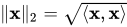
On the -dimensional Euclidean space the intuitive notion of length of the vector is captured by the formula[9]




This is the Euclidean norm, which gives the ordinary distance from the origin to the point X—a consequence of the Pythagorean theorem. This operation may also be referred to as "SRSS", which is an acronym for the square root of the sum of squares.[10]
The Euclidean norm is by far the most commonly used norm on [9] but there are other norms on this vector space as will be shown below. However, all these norms are equivalent in the sense that they all define the same topology on finite-dimensional spaces.
The inner product of two vectors of a Euclidean vector space is the dot product of their coordinate vectors over an orthonormal basis. Hence, the Euclidean norm can be written in a coordinate-free way as
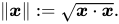
The Euclidean norm is also called the quadratic norm, norm,[11] norm, 2-norm, or square norm; see space. It defines a distance function called the Euclidean length, distance, or distance.


The set of vectors in whose Euclidean norm is a given positive constant forms an -sphere.

Euclidean norm of complex numbers
The Euclidean norm of a complex number is the absolute value (also called the modulus) of it, if the complex plane is identified with the Euclidean plane This identification of the complex number as a vector in the Euclidean plane, makes the quantity (as first suggested by Euler) the Euclidean norm associated with the complex number. For , the norm can also be written as where is the complex conjugate of


Quaternions and octonions
There are exactly four Euclidean Hurwitz algebras over the real numbers. These are the real numbers the complex numbers the quaternions and lastly the octonions where the dimensions of these spaces over the real numbers are respectively. The canonical norms on and are their absolute value functions, as discussed previously.




The canonical norm on of quaternions is defined by for every quaternion in This is the same as the Euclidean norm on considered as the vector space Similarly, the canonical norm on the octonions is just the Euclidean norm on





Finite-dimensional complex normed spaces
On an -dimensional complex space the most common norm is


In this case, the norm can be expressed as the square root of the inner product of the vector and itself: where is represented as a column vector and denotes its conjugate transpose.
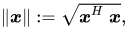

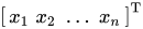

This formula is valid for any inner product space, including Euclidean and complex spaces. For complex spaces, the inner product is equivalent to the complex dot product. Hence the formula in this case can also be written using the following notation:
Taxicab norm or Manhattan norm
The name relates to the distance a taxi has to drive in a rectangular street grid (like that of the New York borough of Manhattan) to get from the origin to the point
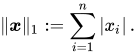

The set of vectors whose 1-norm is a given constant forms the surface of a cross polytope, which has dimension equal to the dimension of the vector space minus 1. The Taxicab norm is also called the norm. The distance derived from this norm is called the Manhattan distance or distance.

The 1-norm is simply the sum of the absolute values of the columns.
In contrast, is not a norm because it may yield negative results.

p-norm
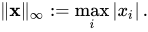
Let be a real number. The -norm (also called -norm) of vector is[9] For we get the taxicab norm, for we get the Euclidean norm, and as approaches the -norm approaches the infinity norm or maximum norm: The -norm is related to the generalized mean or power mean.


For the -norm is even induced by a canonical inner product meaning that for all vectors This inner product can be expressed in terms of the norm by using the polarization identity. On this inner product is the Euclidean inner product defined by while for the space associated with a measure space which consists of all square-integrable functions, this inner product is







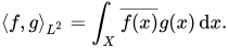
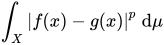
This definition is still of some interest for but the resulting function does not define a norm,[12] because it violates the triangle inequality. What is true for this case of even in the measurable analog, is that the corresponding الفئة هي فضاء متجهي، ومن الصحيح أيضاً أن الدالة (بدونيُعرّف الجذر النوني مسافة تجعلإلى فضاء متجهي طوبولوجي متري كامل . تحظى هذه الفضاءات بأهمية بالغة في التحليل الوظيفي ، ونظرية الاحتمالات ، والتحليل التوافقي . مع ذلك، باستثناء الحالات البسيطة، فإن هذا الفضاء المتجهي الطوبولوجي ليس محدبًا محليًا، ولا يحتوي على أشكال خطية غير صفرية متصلة. وبالتالي، فإن الفضاء الثنائي الطوبولوجي لا يحتوي إلا على الدالة الصفرية.


المشتق الجزئي لـيُعطى المعيار -norm بواسطة
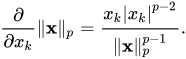
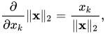
المشتق بالنسبة إلىلذلك، هو أينيشير إلى منتج هادامارد ويُستخدم لحساب القيمة المطلقة لكل عنصر من عناصر المتجه.


في الحالة الخاصة لـيصبح هذا أو

المعيار الأقصى (حالة خاصة من: معيار اللانهاية، أو المعيار الموحد، أو المعيار الأعلى)


لوهو متجه ما بحيثثم:



مجموعة المتجهات التي يكون معيارها اللانهائي ثابتًا معطى،يشكل سطح مكعب فائق بطول حافة


معيار الطاقة
معيار الطاقة [ 13 ] للمتجهيتم تعريفها بدلالة مصفوفة متناظرة موجبة التحديدمثل


من الواضح أنه إذاإذا كانت مصفوفة الوحدة ، فإن هذا المعيار يتوافق مع المعيار الإقليدي .إذا كان قطريًا، يُطلق على هذا المعيار أيضًا اسم المعيار الموزون . ويُستنتج معيار الطاقة من الضرب الداخلي المعطى بواسطةل.


بشكل عام، تعتمد قيمة المعيار على نطاق: بالنسبة للمتجهبمعيار إقليدي يساوي واحدًا، فإن قيمةمحصورة من الأسفل والأعلى بأصغر وأكبر القيم الذاتية المطلقة لـعلى التوالي، حيث يتم تحقيق الحدود إذايتطابق مع المتجهات الذاتية (المُعَيَّرة) المناظرة. استنادًا إلى الجذر التربيعي للمصفوفة المتناظرةيمكن كتابة معيار الطاقة لمتجه بدلالة المعيار الإقليدي القياسي على النحو التالي:


المعيار الصفري
في الاحتمالات والتحليل الوظيفي، يُنشئ المعيار الصفري طوبولوجيا مترية كاملة لفضاء الدوال القابلة للقياس وفضاء F للمتتاليات ذات المعيار F.[ 14 ] ونقصد هنابالمعيار Fدالة حقيقية القيمةعلى مساحة F مع مسافةبحيثإن المعيار F الموصوف أعلاه ليس معيارًا بالمعنى المعتاد لأنه يفتقر إلى خاصية التجانس المطلوبة.



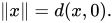
مسافة هامينغ لمتجه من الصفر
في الهندسة المترية ، تأخذ المسافة المتقطعة القيمة واحد للنقاط المتميزة وصفرًا فيما عدا ذلك. عند تطبيقها إحداثيًا على عناصر فضاء متجهي، تُعرّف المسافة المتقطعة مسافة هامينغ ، وهي مهمة في الترميز ونظرية المعلومات . في مجال الأعداد الحقيقية أو المركبة، لا تكون مسافة المسافة المتقطعة من الصفر متجانسة عند النقطة غير الصفرية؛ بل تبقى المسافة من الصفر واحدًا كلما اقترب وسيطها غير الصفري من الصفر. مع ذلك، فإن المسافة المتقطعة لعدد من الصفر تُحقق الخصائص الأخرى للمعيار، وهي متباينة المثلث والتحديد الموجب. عند تطبيقها عنصرًا عنصرًا على المتجهات، تتصرف المسافة المتقطعة من الصفر كمعيار غير متجانس، يحسب عدد العناصر غير الصفرية في وسيط المتجه؛ ومرة أخرى، هذا المعيار غير المتجانس غير متصل.
في معالجة الإشارات والإحصاء ، أشار ديفيد دونوهو إلى " المعيار " الصفري بين علامتي اقتباس. ووفقًا لترميز دونوهو، فإن "المعيار" الصفري لـهو ببساطة عدد الإحداثيات غير الصفرية لـأو مسافة هامينغ للمتجه من الصفر. عندما يتم تحديد هذا "المعيار" لمجموعة محدودة، فإنه يمثل نهاية-norms كـيقترب من الصفر. بالطبع، فإن "المعيار" الصفري ليس معيارًا حقيقيًا، لأنه ليس متجانسًا موجبًا . في الواقع، هو ليس حتى معيارًا من النوع F بالمعنى المذكور أعلاه، لأنه غير متصل، بشكل مشترك ومنفرد، بالنسبة للمتغير القياسي في ضرب عدد قياسي في متجه، وبالنسبة لمتغيره المتجه. وبسبب إساءة استخدام المصطلحات ، يتجاهل بعض المهندسين علامات اقتباس دونوهو ويطلقون بشكل غير مناسب على دالة عدد القيم غير الصفرية اسمالمعيار، الذي يعكس الترميز الخاص بفضاء ليبيغ للدوال القابلة للقياس .

أبعاد لا نهائية
يؤدي تعميم المعايير المذكورة أعلاه إلى عدد لا نهائي من المكونات إلىومساحات لـوفقًا للمعايير


بالنسبة للمتتاليات والدوال ذات القيم المركبة علىعلى التوالي، والتي يمكن تعميمها بشكل أكبر (انظر مقياس هار ). هذه المعايير صالحة أيضًا في النهاية كما، مما يعطي معيارًا أعلى ، ويسمىو


أي منتج داخلي يحفز بشكل طبيعي القاعدة

يمكن العثور على أمثلة أخرى للفضاءات المتجهة المعيارية ذات الأبعاد اللانهائية في مقالة فضاء باناخ .
عموماً، لا تُعطي هذه المعايير نفس البنى الطوبولوجية. على سبيل المثال، بنية لا نهائية الأبعاد space gives a strictly finer topology than an infinite-dimensional space when


Composite norms
Other norms on can be constructed by combining the above; for example is a norm on


For any norm and any injectivelinear transformation we can define a new norm of equal to In 2D, with a rotation by 45° and a suitable scaling, this changes the taxicab norm into the maximum norm. Each applied to the taxicab norm, up to inversion and interchanging of axes, gives a different unit ball: a parallelogram of a particular shape, size, and orientation.

In 3D, this is similar but different for the 1-norm (octahedrons) and the maximum norm (prisms with parallelogram base).
There are examples of norms that are not defined by "entrywise" formulas. For instance, the Minkowski functional of a centrally-symmetric convex body in (centered at zero) defines a norm on (see § Classification of seminorms: absolutely convex absorbing sets below).
All the above formulas also yield norms on without modification.

There are also norms on spaces of matrices (with real or complex entries), the so-called matrix norms.
In abstract algebra
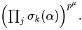
Let be a finite extension of a field of inseparable degree and let have algebraic closure If the distinct embeddings of are then the Galois-theoretic norm of an element is the value As that function is homogeneous of degree , the Galois-theoretic norm is not a norm in the sense of this article. However, the -th root of the norm (assuming that concept makes sense) is a norm.[15]


![{\displaystyle [E:k]}](https://wikimedia.org/api/rest_v1/media/math/render/svg/310a9eea16514b602e0ded65d3ae4ad3dd341938)
Composition algebras
The concept of norm in composition algebras does not share the usual properties of a norm since null vectors are allowed. A composition algebra consists of an algebra over a field an involution and a quadratic form called the "norm".


The characteristic feature of composition algebras is the homomorphism property of : for the product of two elements and of the composition algebra, its norm satisfies In the case of division algebras and the composition algebra norm is the square of the norm discussed above. In those cases the norm is a definite quadratic form. In the split algebras the norm is an isotropic quadratic form.




Properties
For any norm on a vector space تتحقق متباينة المثلث العكسية : لوإذا كانت دالة خطية متصلة بين فضاءات معيارية، فإن معيارومعيار منقولةمتساويان. [ 16 ]



لـ المعايير ، لدينا متباينة هولدر [ 17 ] ومن الحالات الخاصة لذلك متباينة كوشي-شفارتز : [ 17 ]



كل معيار هو شبه معيار، وبالتالي يحقق جميع خصائص المعيار . وبدوره، كل شبه معيار هو دالة شبه خطية ، وبالتالي يحقق جميع خصائص المعيار . وعلى وجه الخصوص، كل معيار هو دالة محدبة .
التكافؤ
يختلف مفهوم دائرة الوحدة (مجموعة جميع المتجهات ذات المعيار 1) باختلاف المعايير: ففي المعيار 1، تكون دائرة الوحدة مربعًا موجهًا على شكل معين؛ وفي المعيار 2 (المعيار الإقليدي)، تكون دائرة الوحدة المعروفة؛ أما في معيار اللانهاية، فتكون مربعًا محاذيًا للمحاور.وفقًا لمعيار -norm، فهو قطع ناقص فائق ذو محاور متطابقة (انظر الرسم التوضيحي المرفق). وبسبب تعريف المعيار، يجب أن تكون دائرة الوحدة محدبة ومتناظرة مركزيًا (لذلك، على سبيل المثال، قد تكون كرة الوحدة مستطيلة ولكن لا يمكن أن تكون مثلثًا، ولـ-norm).
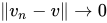
في سياق الفضاء المتجهي، يُعرّف المعيار الجزئي طوبولوجيا على هذا الفضاء، وهي طوبولوجيا هاوسدورف تحديدًا عندما يستطيع المعيار الجزئي التمييز بين متجهات مختلفة، وهو ما يُكافئ كون المعيار الجزئي معيارًا. يمكن فهم الطوبولوجيا المُعرّفة بهذه الطريقة (سواءً بواسطة معيار أو معيار جزئي) إما من حيث المتتاليات أو المجموعات المفتوحة. متتالية من المتجهاتيقال إنها تتقارب في المعيار إلىلومثلبصورة مكافئة، تتكون الطوبولوجيا من جميع المجموعات التي يمكن تمثيلها كاتحاد كرات مفتوحة . إذاإذا كان فضاءً معياريًا [ 18 ]




![{\displaystyle \|xy\|=\|xz\|+\|zy\|{\text{ لجميع }}x,y\in X{\text{ و }}z\in [x,y].}](https://wikimedia.org/api/rest_v1/media/math/render/svg/260066e13f1afcce833e2deda11b06fce7662378)
معيارانوفي فضاء متجهيتم الاتصال بـتكون متكافئة إذا أدت إلى نفس البنية الطوبولوجية، [ 19 ] وهو ما يحدث إذا وفقط إذا وُجدت أعداد حقيقية موجبةوبحيث يكون ذلك لجميع على سبيل المثال، إذاعلىثم [ 20 ]





بخاصة، إنه، إذا كان الفضاء المتجهي حقيقيًا أو مركبًا محدود الأبعاد، فإن جميع المعايير تكون متكافئة. أما في حالة الفضاءات المتجهة غير المحدودة الأبعاد، فلا تكون جميع المعايير متكافئة.




تُعرّف المعايير المتكافئة نفس مفاهيم الاستمرارية والتقارب، ولا داعي للتمييز بينها في كثير من الأحيان. بتعبير أدق، فإن البنية المنتظمة التي تُعرّفها المعايير المتكافئة على فضاء المتجهات متماثلة بشكل منتظم . يجب ألا يُفهم من هذا التكافؤ أن المعايير قابلة للتبادل دائمًا. ففي سياق ملاءمة النماذج، على سبيل المثال، قد تؤدي المعايير المختلفة إلى نتائج ملاءمة مختلفة وكفاءات خوارزمية متباينة.
تصنيف المعايير شبهية: مجموعات محدبة مطلقة ماصة
جميع المعايير شبهية على فضاء متجهييمكن تصنيفها من حيث المجموعات الفرعية المحدبة المطلقة الماصةللكل مجموعة فرعية من هذا القبيل معيار شبهييُطلق عليه مقياسيُعرَّف بأنه أينهو الحد الأدنى ، وله الخاصية التي وعلى العكس:




أي فضاء متجهي طوبولوجي محدب محليًا له أساس محلي يتكون من مجموعات محدبة مطلقًا. إحدى الطرق الشائعة لإنشاء مثل هذا الأساس هي استخدام عائلةمن المعايير شبه القياسيةالتي تفصل النقاط : مجموعة جميع التقاطعات المحدودة للمجموعاتيحول الفضاء إلى فضاء متجهي طوبولوجي محدب محليًا بحيث يكون كل p متصلًا .


تُستخدم هذه الطريقة لتصميم الطوبولوجيات الضعيفة والضعيفة* .
الحالة العادية:
- لنفترض الآن أنيحتوي على واحدمنذينفصلان ،هذا أمر طبيعي، وهي كرة الوحدة المفتوحة . ثمهي جوار محدب ومحدود تمامًا للصفر، ومتصل.

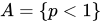

- أما العكس فيعود إلى أندريه كولموغوروف : أي فضاء متجهي طوبولوجي محدب محليًا ومحدود محليًا يكون قابلاً للتطبيع . تحديدًا:
- لوهي جوار محدب ومحدود تمامًا للصفر، وهو المقياس(لهذا السببهذا أمر طبيعي.

انظر أيضاً
- المعيار غير المتماثل – تعميم لمفهوم المعيار
- شبه المعيار F - فضاء متجهي طوبولوجي يمكن تعريف طوبولوجيته بواسطة مقياس. صفحات تعرض أوصافًا موجزة لأهداف إعادة التوجيه
- معيار غاورز – فئة من المعايير في التوافقية الجمعية
- معيار كاديك – جميع فضاءات باناخ اللانهائية الأبعاد والقابلة للفصل متماثلة الشكل. صفحات تعرض أوصافًا موجزة لأهداف إعادة التوجيه
- تحليل الطيف باستخدام طريقة المربعات الصغرى – طريقة حساب الدورية
- مسافة ماهالانوبيس – مقياس المسافة الإحصائية
- المقدار (في الرياضيات) – خاصية تحدد المقارنة والترتيب
- معيار المصفوفة – المعيار على فضاء متجهي من المصفوفات
- مسافة مينكوفسكي - دالة المسافة المتجهة
- وظيفة مينكوفسكي - وظيفة مصنوعة من مجموعة
- معيار المؤثر – مقياس "حجم" المؤثرات الخطية
- بارانورم - فضاء متجهي طوبولوجي يمكن تعريف طوبولوجيته بواسطة مقياس. صفحات تعرض أوصافًا موجزة لأهداف إعادة التوجيه
- العلاقة بين المعايير والمقاييس – الفضاء الرياضي مع مفهوم المسافة. صفحات تعرض أوصافًا موجزة لأهداف إعادة التوجيه.
- شبه المعيار - دالة رياضية
- الدالة شبه الخطية - نوع من الدوال في الجبر الخطي
ملحوظات
- ↑ تلميح: في الخاصية (1.)، استخدم.

مراجع
- 1 2 كناب، أ. و. (2005). التحليل الحقيقي الأساسي . بيركهاوزر. ص. رقم الكتاب المعياري الدولي ( ISBN) 978-0-817-63250-2.
- ↑ "Pseudonorm" . www.spektrum.de (بالألمانية) . تم الاطلاع عليه بتاريخ 12-05-2022 .
- ↑ هايرز، د. هـ. (1939-09-01). "الفضاءات الخطية شبه المعيارية والمجموعات الأبيلية" . مجلة ديوك الرياضية . 5 (3). doi : 10.1215/s0012-7094-39-00551-x . ISSN 0012-7094 .
- ↑ بو، سي سي (2015). التحليل الرياضي الحقيقي . سبرينغر. ص. صفحة 28. ISBN 978-3-319-17770-0.بروغوفيتشكي، إي. (1981). ميكانيكا الكم في فضاء هيلبرت . ص. الصفحة 20 .
- 1 2 كوبروسلي 2011 ، ص. 200.
- ↑ رودين، و. (1991). التحليل الوظيفي . ص 25.
- ↑ ناريسي وبيكنشتاين 2011 ، ص 120-121.
- ↑ ويلانسكي 2013 ، ص 20-21.
- 1 2 3 وايسشتاين، إريك دبليو. "معيار المتجه" . mathworld.wolfram.com . تم الاسترجاع في 24 أغسطس 2020 .
- ↑ تشوبرا، أنيل (2012). ديناميكيات الهياكل، الطبعة الرابعة . برنتيس هول. ISBN 978-0-13-285803-8.
- ↑ وايسشتاين، إريك دبليو. "نورم" . mathworld.wolfram.com . تم الاطلاع عليه بتاريخ 24 أغسطس 2020 .
- ↑ باستثناء فيحيث يتطابق مع المعيار الإقليدي، وحيث يكون الأمر تافهاً.
- ↑ سعد، يوسف (2003)، الطرق التكرارية للأنظمة الخطية المتفرقة ، ص 32، ISBN 978-0-89871-534-7
- ↑ روليفيتش، ستيفان (1987)، التحليل الوظيفي ونظرية التحكم: الأنظمة الخطية ، الرياضيات وتطبيقاتها (سلسلة أوروبا الشرقية)، المجلد 29 (ترجمة من البولندية بواسطة إيفا بيدنارتشوك، محررة)، دوردريخت؛ وارسو: دار نشر دي. ريدل؛ PWN - الناشرون العلميون البولنديون، الصفحات 16، 524، doi : 10.1007/978-94-015-7758-8 ، ISBN 90-277-2186-6، MR 0920371 ، OCLC 13064804
- ^ لانج، سيرج (2002) [1993]. الجبر (الطبعة الثالثة المنقحة ). نيويورك: سبرينغر فيرلاغ. ص. 284. ردمك 0-387-95385-X.
- ^ تريف 2006 ، ص 242-243.
- 1 2 غولوب، جين ؛ فان لون، تشارلز ف. (1996). حسابات المصفوفات ( الطبعة الثالثة). بالتيمور: مطبعة جامعة جونز هوبكنز. ص 53. ISBN 0-8018-5413-X.
- ↑ ناريسي وبيكنشتاين 2011 ، ص 107-113.
- ↑ كونراد، كيث. "تكافؤ المعايير" (ملف PDF) . kconrad.math.uconn.edu . تم الاطلاع عليه في 7 سبتمبر 2020 .
- ↑ "العلاقة بين المعايير p" . موقع تبادل الأسئلة والأجوبة في الرياضيات .


فهرس
- بورباكي، نيكولا (1987) [1981]. مساحات المتجهات الطوبولوجية: الفصول 1-5 . عناصر الرياضيات . تمت الترجمة بواسطة Eggleston، HG. مادان، س. برلين نيويورك: سبرينغر-فيرلاغ. رقم ISBN 3-540-13627-4. OCLC 17499190 .
- خليل الله، إس إم (1982). أمثلة مضادة في فضاءات المتجهات الطوبولوجية . سلسلة محاضرات في الرياضيات . المجلد 936. برلين، هايدلبرغ، نيويورك: سبرينغر-فيرلاغ . ISBN 978-3-540-11565-6. OCLC 8588370 .
- كوبروسلي، كارلوس س. (2011). عناصر نظرية المؤثرات ( الطبعة الثانية). بوسطن: بيركهاوزر . ISBN 978-0-8176-4998-2. OCLC 710154895 .
- ناريسي، لورانس؛ بيكنشتاين، إدوارد (2011). فضاءات المتجهات الطوبولوجية . الرياضيات البحتة والتطبيقية ( الطبعة الثانية). بوكا راتون، فلوريدا: مطبعة سي آر سي. رقم ISBN 978-1584888666. OCLC 144216834 .
- شيفر، هيلموت هـ .؛ وولف، مانفريد ب. (1999). فضاءات المتجهات الطوبولوجية . سلسلة GTM . المجلد 8 ( الطبعة الثانية). نيويورك، نيويورك: سبرينغر نيويورك. رقم ISBN 978-1-4612-7155-0. OCLC 840278135 .
- تريف، فرانسوا (2006) [1967]. فضاءات المتجهات الطوبولوجية والتوزيعات والنوى . مينيولا، نيويورك: منشورات دوفر. رقم ISBN 978-0-486-45352-1. OCLC 853623322 .
- ويلانسكي، ألبرت (2013). الأساليب الحديثة في فضاءات المتجهات الطوبولوجية . مينولا، نيويورك: منشورات دوفر. ISBN 978-0-486-49353-4. OCLC 849801114 .
- التحليل الوظيفي
- الجبر الخطي
- المعايير (الرياضيات)